# Marine sub-sediment burial

| **Module name**      | Marine sub-sediment burial                 |
| -------------------- | ------------------------------------------ |
| **Module category**  | Carbon storage                             |
| **Methodology nam**e | Biomass carbon removal and storage (BiCRS) |
| **Version**          | 1.0                                        |
| **Methodology ID**   | RBW-BICRS-CS-MSSB-V1.0                     |
| **Release date**     | August 28th, 2025                          |
| **Status**           | In use                                     |

{% content-ref url="../../../glossary" %}
[glossary](https://docs.rainbowstandard.io/~/changes/113/glossary)
{% endcontent-ref %}

<details>

<summary>Acknowledgements <span data-gb-custom-inline data-tag="emoji" data-code="1f91d">🤝</span></summary>

This module was developed by Rainbow with support from [Sinkco Labs](https://www.sinkcolabs.com/), particularly their science team, Brenna Boehman (Ph.D.) and Daniel Babin (Ph.D.), who provided fundamental scientific knowledge on storage in sub-sediment anoxic conditions. We extend our gratitude to [EcoEngineers ](https://www.ecoengineers.us/)and [David Harning, PhD](https://www.colorado.edu/instaar/david-harning), for their expert review. Rainbow sincerely appreciates the valuable contributions of all involved in this work.

</details>

This is a **Carbon Storage Module** and covers Marine sub-sediment burial. This module is part of the Rainbow BiCRS methodology, which allows Project Developers to choose the relevant modules for their project, and shall be used with the necessary accompanying modules.

See more details on how modules are organized in the [BiCRS home page](https://docs.rainbowstandard.io/~/changes/113/methodologies/biomass-carbon-removal-and-storage-bicrs/..#efpqng3v3ute).

<table data-view="cards" data-full-width="false"><thead><tr><th></th><th></th><th></th><th data-hidden data-card-target data-type="content-ref"></th><th data-hidden data-card-cover data-type="files"></th></tr></thead><tbody><tr><td><strong>How to use this module</strong></td><td></td><td></td><td><a href="../..#efpqng3v3ute">#efpqng3v3ute</a></td><td><a href="https://1461901304-files.gitbook.io/~/files/v0/b/gitbook-x-prod.appspot.com/o/spaces%2FE1FUJsBoIj20nqp3CtMf%2Fuploads%2FWRAnXQMFNSn97t9GOrFx%2Fpexels-eberhardgross-1612461.jpg?alt=media&#x26;token=2c97e54f-1b97-4eb7-aead-e423aea08c21">pexels-eberhardgross-1612461.jpg</a></td></tr><tr><td><strong>BiCRS Methodology</strong></td><td></td><td></td><td><a href="..">..</a></td><td><a href="https://1461901304-files.gitbook.io/~/files/v0/b/gitbook-x-prod.appspot.com/o/spaces%2FE1FUJsBoIj20nqp3CtMf%2Fuploads%2FR0TN0FvXWcrjcVsSjXI1%2Fbiochar.png?alt=media&#x26;token=53fc0925-3647-46c4-9485-01a72039cebe">BiCRS methodology.png</a></td></tr></tbody></table>

## Eligible technologies

#### Project type <a href="#uikucys7r1rk" id="uikucys7r1rk"></a>

This module covers marine sub-sediment burial projects that inject waste and residual biomass feedstock inputs directly into the [**anoxic** ](#user-content-fn-1)[^1]layer of [marine sub-sediments](#user-content-fn-2)[^2]. Projects shall meet all of the following criteria:

* Demonstrate capability to perform MRV as agreed upon in the validated project documentation
* Demonstrate a net-negative project carbon footprint based on initial LCA estimates of induced emissions and initial CDR estimates based on modeling
* Projects that **sink** biomass to the seafloor but do not bury and embed it into marine sub-sediments are **not eligible**.
* The entity eligible for receiving carbon finance is the operator performing storage at the sub-sediment burial site. Biomass producers and sub-sediment burial machinery manufacturers are not eligible Project Developers.

#### Project scope <a href="#gs84uiswpg2k" id="gs84uiswpg2k"></a>

A project is defined as **all burial activities that take place from one port** over the project lifetime (by default a maximum of 5 years, [renewable](https://docs.rainbowstandard.io/~/changes/113/rainbow-standard-documents/procedures-manual/project-certification-procedure#crediting-period-renewal)), and all removal that occurs as a result of that burial, plus the upstream/downstream activities associated with that burial (e.g. GHG emissions from feedstock sourcing, transport...).

See the [Storage batch](#ad7rimjzuv5e) section for more details on how a project is organized into different burial areas and burial events.

#### Eligible sites <a href="#aih0rwwz5szx" id="aih0rwwz5szx"></a>

Storage must be done in [**anoxic** ](#user-content-fn-1)[^1]conditions.

Storage must be done in **existing accessible** [**marine sub-sediment**](#user-content-fn-2)[^2]. Projects that excavate, dredge or build wells for the sole purpose of accessing sub-sediments or creating sub-sediment conditions are not eligible, due to the associated environmental risks.

See the [Site characterization](#id-9yt6lk62t36) section for more specific requirements.

#### Eligible feedstock <a href="#ja1qpxfjotc" id="ja1qpxfjotc"></a>

Only [particulate terrestrial biomass](#user-content-fn-3)[^3] feedstock that also meets the requirements of the[ BiCRS Biomass Feedstock module](https://docs.rainbowstandard.io/~/changes/113/methodologies/biomass-carbon-removal-and-storage-bicrs/carbon-capture/biomass-feedstock) is eligible in this module. Injection of liquefied or gaseous CO$$\_2$$ into sediments is outside the scope of this module.

See the [BiCRS Biomass Feedstock module](https://docs.rainbowstandard.io/~/changes/113/methodologies/biomass-carbon-removal-and-storage-bicrs/carbon-capture/biomass-feedstock) for more specific feedstock requirements.

## Crediting timeline and process <a href="#vqih1nxeqk4n" id="vqih1nxeqk4n"></a>

{% stepper %}
{% step %}

#### Pre-project sampling

Before or in parallel to validation with Rainbow, the Project Developer shall obtain the necessary permits, and take measurements and samples, and gather secondary sources, for the [Site Characterization Report](#id-9yt6lk62t36-1) and feedstock characterization, and propose a [sampling plan](#aklb6qbc2jek).&#x20;
{% endstep %}

{% step %}

#### Project validation

The Project Developer submits required documentation and undergoes an ex-ante validation audit. The project documentation is made available on the registry, and expected CDR volume is estimated and displayed for pre-purchase agreements. Specific prerequisites include:

* [Permissions ](#o97hd5b4ge3i)have been granted to operate at the storage site, and to monitor the site up to 12-months after storage.
* The storage points are technically appropriate and can allow for permanent carbon storage. This is proven by generating the [Site Characterization Report](#id-9yt6lk62t36-1), demonstrating adherence to all requirements in the [Storage site requirements](#id-9yt6lk62t36-1) section.
* The biomass feedstock has been secured and a preliminary assessment of organic carbon content has been made.
* Expected project-scale CDR is modeled using equations in the [GHG quantification](https://docs.rainbowstandard.io/~/changes/113/methodologies/battery-second-life/ghg-quantification) section.&#x20;
  {% endstep %}

{% step %}

#### Burial events

The feedstock mixture is buried in the predefined storage points. Visual proof of each burial event and site closure is required, via imagery documented and verified in Monitoring Reports, to confirm that the site is well-sealed by surrounding sediments or other surface enhancements (e.g. rocks/rubble, clay caps) and confirm closure.
{% endstep %}

{% step %}

#### (Optional) Monitoring: first measurement, verification and credit issuance

Between 1-3 months after burial, Project Developers may conduct first monitoring by following the [Monitoring Plan](#snhouoxhyrzi) and the [Sampling Plan](#aklb6qbc2jek) to measure organic carbon content in buried biomass for each storage batch. Additional storage points may be added within the validated storage sites. CDR estimates and permanence are [updated with verified real data](#bpf7f2gx9dj5).

Project Developers may choose to either use:

* **50/50 issuance:** undergo a verification audit by a VVB at the first measurement step and issue the first 50% of removal RCCs on the Rainbow registry. Repeat the audit after the following step (Step 5) to issue the remaining 50%, or&#x20;
* **One-time issuance:** skip this first measurement and verification step, and wait to issue 100% of RCCs at the second measurement stage described below (Step 5).
  {% endstep %}

{% step %}

#### Monitoring: second measurement, verification and credit issuance

Project Developers conduct the second monitoring at least 12 months after burial, following the [Monitoring Plan](#snhouoxhyrzi) and the [Sampling Plan](#aklb6qbc2jek), to measure organic carbon content in buried biomass for each storage batch. CDR estimates and permanence are [updated with verified real data](#bpf7f2gx9dj5), and verified by the VVB.

* **50/50 issuance:** the remaining credits are issued. Any discrepancies in earlier results, for example as a result of degradation, shall be accounted for by updating CDR calculations and following the [over/under crediting mechanism](https://docs.rainbowstandard.io/~/changes/113/rainbow-standard-documents/procedures-manual/rcc-management-avoiding-over-crediting#under-overachievement) in the Rainbow Procedures Manual.
* **One-time issuance:** all credits are issued for that storage batch based on the 12-month measurements.
  {% endstep %}

{% step %}

#### Ongoing project operations

Steps 3 through 5 are repeated throughout the 5-year project crediting period for as many storage batches as the Project Developer completes.&#x20;
{% endstep %}

{% step %}

#### End of project and renew the crediting period

Monitoring and verification continues for a maximum of 5 years until the end of the crediting period. The Project Developer may choose to [renew the project's crediting period](https://docs.rainbowstandard.io/~/changes/113/rainbow-standard-documents/procedures-manual/project-certification-procedure#crediting-period-renewal) to extend the Monitoring Plan and continue repeating steps 3 through 5.
{% endstep %}
{% endstepper %}

## Storage batches <a href="#ad7rimjzuv5e" id="ad7rimjzuv5e"></a>

Measurements and reporting are performed for **storage batches**. Verification and credit issuance is done at the reporting period scale (by default, annually), and groups results for all storage batches concerned during that reporting period. The organization of a project into **storage batches**, **sites** and **points** is described below, and depicted in Figure 1.

<table data-view="cards"><thead><tr><th></th></tr></thead><tbody><tr><td>A <strong>storage batch</strong> is all burial events of homogenous feedstock mixtures at one storage site over a maximum of 31 days.</td></tr><tr><td>A <strong>storage site</strong> is a group of similar storage points within 24 km<span class="math">^2</span> of one another with similar site characteristics.</td></tr><tr><td>A <strong>storage point</strong> is the precise spot where a burial event occurs. Similar storage points may be grouped into a storage site.</td></tr></tbody></table>

<figure><img src="https://1461901304-files.gitbook.io/~/files/v0/b/gitbook-x-prod.appspot.com/o/spaces%2FE1FUJsBoIj20nqp3CtMf%2Fuploads%2Fn79BB33ec2pTAM3XT8Rh%2FClimate%20team%20-%20Schemes%20-%20Frame%205%20(1).jpg?alt=media&#x26;token=1a28a2de-eb69-47c6-a57a-d10a8e401263" alt=""><figcaption><p>Figure 1 This figure illustrates how a project is organized into storage batches, storage sites, and storage points. Storage Batch #1 and Storage Batch #2 differ because Storage Batch #1 exceeded the 31-day limit and rolled over into a new batch. Storage Batch #1 and Storage Batch #3 occur over the same dates but are stored at different sites under distinct conditions. Meanwhile, Storage Batch #3 and Storage Batch #4 represent a shift in feedstock mixture, which defines a new storage batch, even though the previous batch did not reach the full 31-day duration.</p></figcaption></figure>

Sedimentary conditions for storage points within one storage site must be within the following ranges (data requirements are outlined in the [Data Sources](#g6ohrisnjsbj) section):

* **Grain size:** Grain size must be predominantly (> 50%) mud (< 63 µm grain size in diameter)
* **Water depth** at storage point: At water depths 1-20 m, water depths must be within 0.5 m. At water depths 20-200 m, water depths must be within 5 m.
* **Sub-sediment depth** of storage: At sub-sediment depths 2-3 m, storage depths must be within 0.5 m. At sub-sediment depths >3 m, storage depths must be within 1 m.

Ongoing burial into the sub-sediment shall last no longer than [**31 days per storage batch**](#user-content-fn-4)[^4], to standardize sampling timescales. If burial continues after 31 days, it shall be considered a separate storage batch.

One project may work with different storage batches simultaneously. **Each storage batch shall be monitored and reported separately** within the same Monitoring Report. Storage batch information shall be monitored and reported at least once per calendar year.

Information about storage batches may be monitored and [**issued credits continuously**](https://docs.rainbowstandard.io/~/changes/113/rainbow-standard-documents/procedures-manual/project-certification-procedure#continuous-issuance) by Project Developers by uploading claim information to the Rainbow MRV platform.

## Feedstock mixture <a href="#id-9yt6lk62t36" id="id-9yt6lk62t36"></a>

A feedstock mixture is defined as one biomass feedstock or uniform mixtures of feedstocks. One feedstock mixture may be used across several storage batches, but any time the feedstock mixture of one storage batch changes, a new storage batch shall be started.

Any water used in the feedstock mixture must come from within the 24 km$$^2$$ storage batch area.

The feedstock mixture composition may vary by no more than 20% to be considered the same homogeneous feedstock mixture, where the composition is made of feedstocks of a specific type from a specific supplier.

See the [Pre-burial sampling](#pre-burial-sampling) section for requirements on feedstock sampling.

{% hint style="info" %}
For example, if a feedstock mixture is composed of 50% sawdust and 50% shredded straw, the proportions can vary between 40% and 60% (±10% of the original 50% for both inputs).

If a feedstock mixture is composed of 50% sawdust from Supplier A and and 50% from Supplier B, the proportions can vary between 40% and 60% (±10% of the original 50% for both inputs).
{% endhint %}

## Storage site and storage point requirements <a href="#id-9yt6lk62t36" id="id-9yt6lk62t36"></a>

Storage points must meet the criteria outlined in Table 1 to be eligible. The criteria are set to ensure storage points are suitable for permanent carbon storage, are anoxic, and have low reversal risks.

All criteria shall be outlined in the **Site Characterization Report**, prepared before any burial events occur and submitted with the PDD for the validation audit. In addition, the Site Characterization Report shall provide GPS coordinates of each planned storage point, and a GIS-generated map showing each storage point and the delineation of the associated storage site.

{% hint style="info" %}
Additional storage sites and points may be proposed after project operations begin and credits are issued, provided no burial occurs at the new sites or points before they are validated. To add new storage sites and points, the Project Developer must update the Site Characterization Report with the required details. A VVB shall audit the report to ensure compliance with requirements in Table 1. Once approved, the new sites and points must adhere to the monitoring plan requirements.
{% endhint %}

Data sources characterizing storage points must be, in the following order of preference:

1. primary data from a pilot survey e.g. site surveys, in situ measurements and measurements on samples collected at the project site, delivered by the Project Developer, or
2. secondary data from the specific area concerned (e.g. published peer-reviewed literature or database measurements) or
3. secondary data from an area that is proven to be sufficiently representative and similar to the project area in the appropriate factors that relate to permanent storage.

*Table 1 The required measurements and information for a storage site that must be presented in the Site Characterization Report, before any burial occurs, to justify that the storage site is appropriate for permanent CDR via marine sub-sediment burial.*

<table><thead><tr><th width="162">Criteria</th><th>Description</th></tr></thead><tbody><tr><td><strong>Marine water</strong></td><td>Must be in coastal, sea or ocean waters with a salinity greater than zero. Freshwater burial is not currently eligible.
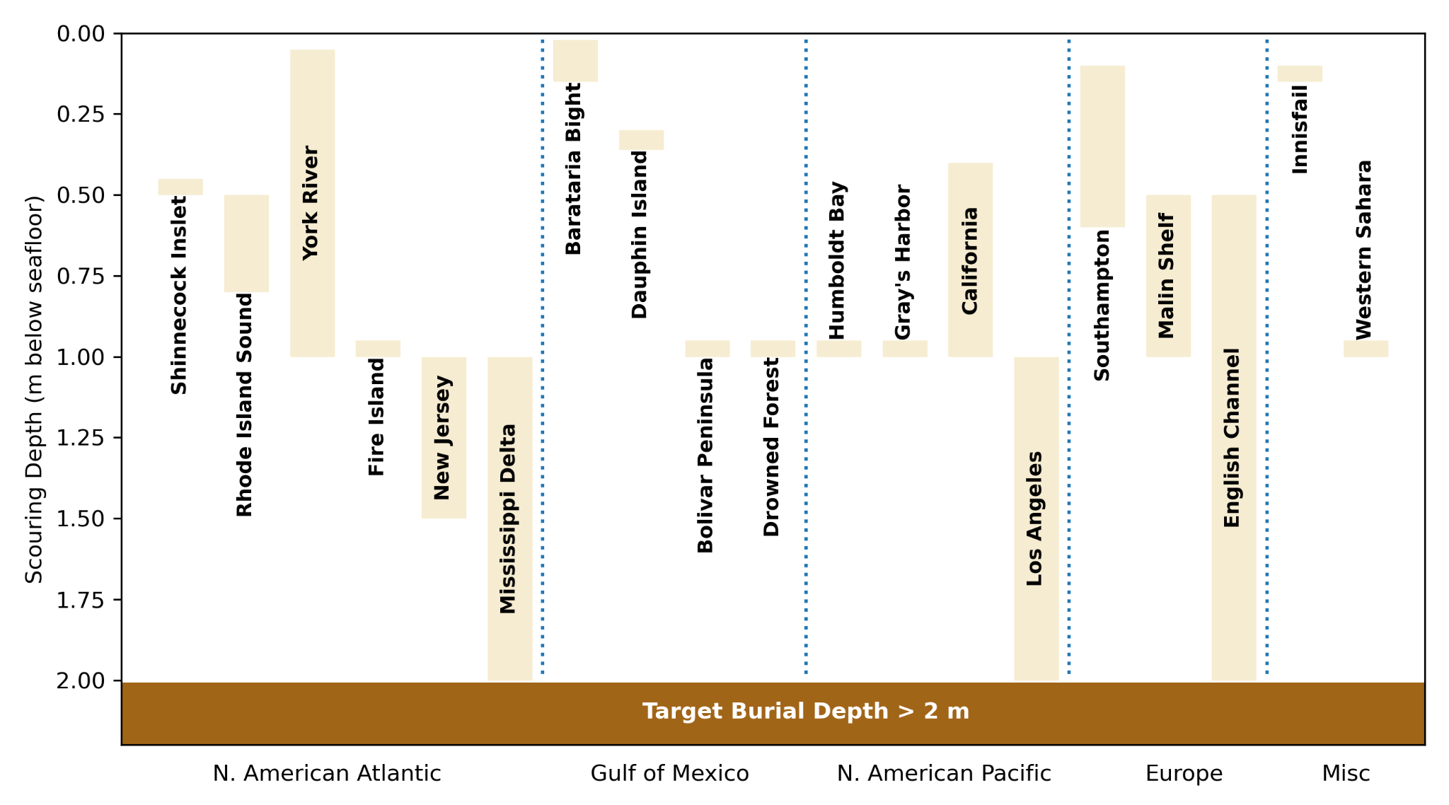
 </td></tr><tr><td><strong>Anoxic Sediment Layer</strong></td><td><p>Must reach deep enough into the sub-sediment to reach the <a data-footnote-ref href="#user-content-fn-2">anoxic zone</a>. This shall be <strong>at least 2 m into the sediment</strong> (see <a href="#dg5ezfux812d">Appendix </a>D for justification), but actual depth to achieve this varies by site and shall be justified for each project. </p><p>The depth must remain anoxic year-round, accounting for bioturbation or increased advection/diffusion into sediments. The sub-sediment area must be stable with low likelihood of re-exposure, proven via established tools for determining sediment stability such as 210Pb or other geochronology tools.</p></td></tr><tr><td><strong>Water depth</strong></td><td>Must ensure the surface of the water bottom (seafloor or sediment surface) is not exposed to the air during tidal fluctuations. At water depths 1-20 m, water depths must be within 0.5 m. At water depths 20-200 m, water depths must be within 5 m</td></tr><tr><td><strong>Methane diffusion</strong></td><td>Methane must not be diffusing out of the sediment-water interface. This is measured using <a data-footnote-ref href="#user-content-fn-5">oxygen penetration depth</a> as a proxy for methane diffusion. This requirement is to ensure that if any buried feedstock mixture degrades, it would not be emitted as the stronger GHG methane, and would instead  be emitted as CO<span class="math">_2</span>. In any case, loss of organic carbon from the biomass would be detected.
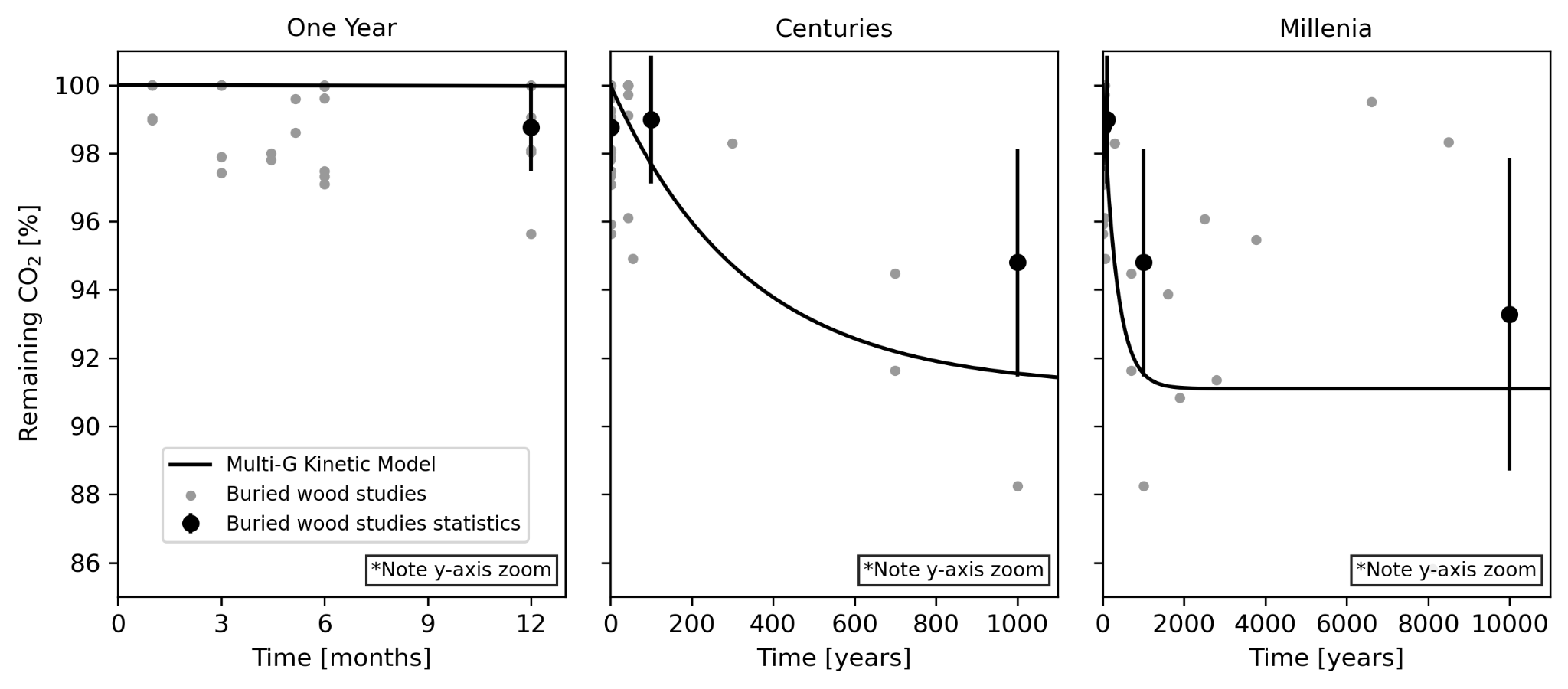
</td></tr><tr><td><strong>Potential gas exchange</strong></td><td><p>Project Developers shall use all criteria mentioned above to calculate potential gas exchange from embedded depth into the atmosphere, to justify that there will be minimal gas exchange of any evolved gases with the atmosphere during a 1000 year period. </p><p>This requirement ensures that if any buried feedstock mixture degrades, the CO<span class="math">_2</span> generated will likely remain trapped in the sediment and remain stored, rather than <a data-footnote-ref href="#user-content-fn-6">diffusing </a>through the water column into the atmosphere.</p></td></tr><tr><td><strong>Shelf slope</strong></td><td>Sediment or seafloor gradation must be &#x3C;1:100 to prevent sediment <a data-footnote-ref href="#user-content-fn-7">slumping</a>.</td></tr><tr><td><strong>Sediment grain size</strong></td><td>At the target sub-sediment depth, at least 50% of sediment grains must be maximum 63 µm particle size.</td></tr><tr><td><strong>Authorization and access</strong></td><td>Project Developers must be authorized by jurisdictional authorities to operate, perform burial events and complete monitoring at the given geographic coordinates.</td></tr><tr><td><strong>Potential for Future Disturbance</strong></td><td>This shall be qualitatively and transparently discussed in the Site Characterization Report to determine if sediment disturbance may occur in the next 40 years, due to deep-sea mining, oil and gas extraction, trawling from fishing vessels, other resource exploitation, or any other use-conflict that might lead to reversal of storage. The site lease agreement should implement suitable barriers to such disturbance events.</td></tr><tr><td><strong>Marine life</strong></td><td>Characterize the biodiversity of marine life at the storage site, considering species type and abundance. This is used to 1) identify any sensitive biodiversity hotspots and 2) as a benchmark to compare identify any environmental damages after post-burial. Jurisdictional permitting and Environmental Impact Assessment procedures should already cover this, so this is implemented as an abundance of caution. </td></tr></tbody></table>

## Sampling requirements <a href="#aklb6qbc2jek" id="aklb6qbc2jek"></a>

Sampling occurs at two stages of the project: sampling of the feedstock mixture before burial to establish organic carbon buried, and sampling the feedstock mixture after burial to check for any reversals (i.e. carbon degradation or diffusion). At both stages of sampling, laboratory testing shall provide the following measurements of the feedstock mixture:

* % organic carbon content of the solid biomass
* % moisture content of the feedstock mixture
* density of the feedstock mixture

### **Pre-burial sampling**

Two representative samples of the feedstock mixture shall be prepared and sent for laboratory testing per storage batch: one at the beginning (day one) and one at the end of the storage batch (day 31, or an earlier date when the storage batch is complete).

### **Post-burial monitoring and sampling**

Post-burial monitoring and sampling shall occur:

* at least 12 months after the burial event, and
* optionally, may also be performed within 1-3 months after the burial event if the Project Developer chooses the 50/50 credit issuance approach. See the [Crediting timeline and process ](#vqih1nxeqk4n)section for more details.

Post-burial monitoring and sampling should be completed using sediment coring, to access the buried biomass, extract samples, and send them to a laboratory to measure the organic content of the solid biomass. Alternative approaches may be considered on a case by case basis, and approved by the VVB, the Rainbow Certification team and, if deemed necessary by the Rainbow Certification team, an expert peer reviewer.

**Sampling and laboratory testing shall be done separately for each storage point**. At least three sub-samples shall be taken from each storage point and mixed together to obtain one composite sample for the storage point. Samples can not be mixed from all storage points in one storage site to perform laboratory tests on a composite sample.

### Sampling plan

Project Developers shall prepare an **ex-ante** **Sampling Plan** before any burial events occur, and submit it with the PDD for the validation audit. The Sampling Plan shall describe:

* how representative samples will be taken of the feedstock mixture in pre-burial sampling
* how to preserve moisture content of feedstock mixture while sending it to the lab
* number of samples used for post-burial sampling
* strategy for ensuring random/representative/unbiased sampling locations for post-burial sampling

### **Sampling procedure**

The Sampling Plan described above is developed ex-ante during validation and outlines the *intended* sampling approach. During monitoring and ex-post verification, Project Developers must provide a **Sampling Procedure**, described in the [Monitoring Report](https://docs.rainbowstandard.io/~/changes/113/rainbow-standard-documents/procedures-manual/project-certification-procedure#monitoring-plan), which documents the actual sampling approach that was implemented.

Ideally, the Sampling Procedure should align exactly with the Sampling Plan. However, given real-world challenges that may arise during monitoring, deviations are expected. The purpose of documenting the Sampling Procedure ex-post is to ensure transparency by capturing any adjustments made to the original plan.

The **Sampling Procedure shall include all elements listed in the Sampling Plan components** section.

## Eligibility criteria <a href="#id-8818d1p2uq2v" id="id-8818d1p2uq2v"></a>

The eligibility criteria requirements specific to this module are detailed in the sections below. Other eligibility criteria requirements shall be taken from the accompanying modules and methodologies:

<table data-view="cards"><thead><tr><th></th><th></th><th></th><th data-hidden data-card-target data-type="content-ref"></th><th data-hidden data-card-cover data-type="files"></th></tr></thead><tbody><tr><td><strong>BiCRS methodology</strong></td><td><ul><li>Additionality</li><li>No double counting</li><li>Targets alignment</li><li>ESDNH</li></ul></td><td></td><td><a href="..">..</a></td><td><a href="https://1461901304-files.gitbook.io/~/files/v0/b/gitbook-x-prod.appspot.com/o/spaces%2FE1FUJsBoIj20nqp3CtMf%2Fuploads%2FR0TN0FvXWcrjcVsSjXI1%2Fbiochar.png?alt=media&#x26;token=53fc0925-3647-46c4-9485-01a72039cebe">BiCRS methodology.png</a></td></tr><tr><td><strong>Other modules</strong></td><td><ul><li>Substitution</li><li>Co-benefits</li><li>No double counting</li><li>ESDNH</li><li>Leakage</li></ul></td><td></td><td><a href=""></a></td><td><a href="https://1461901304-files.gitbook.io/~/files/v0/b/gitbook-x-prod.appspot.com/o/spaces%2FE1FUJsBoIj20nqp3CtMf%2Fuploads%2FF1IanyzrKsw31BYTsPoH%2Ffre-sonneveld-q6n8nIrDQHE-unsplash.jpg?alt=media&#x26;token=208fac4c-8056-41fd-b7c3-1bb14c9e20a2">energy co products module.jpg</a></td></tr><tr><td><strong>Rainbow Standard Rules</strong></td><td><ul><li>Measurability</li><li>Real</li><li>TRL</li><li>Minimum impact</li></ul></td><td></td><td><a href="https://github.com/riverse-carbon/standard-documentation/blob/main/methodologies/biomass-carbon-removal-and-storage-bicrs/carbon-storage/broken-reference/README.md">https://github.com/riverse-carbon/standard-documentation/blob/main/methodologies/biomass-carbon-removal-and-storage-bicrs/carbon-storage/broken-reference/README.md</a></td><td></td></tr></tbody></table>

### Permanence <a href="#id-6mhy92a80ym0" id="id-6mhy92a80ym0"></a>

Removal Rainbow Carbon Credits (RCCs) issued from marine sub-sediment burial have a permanence horizon of 1000 years.

Permanence is assessed at two points during project certification:

* at ex-ante validation it is **estimated using site requirements that identify suitable sites for permanent burial**
* during verification it is **demonstrated using direct measurements**.&#x20;

Requirements for each stage are detailed below.

#### Estimating permanence at validation <a href="#k1tsrh5yuegy" id="k1tsrh5yuegy"></a>

To demonstrate that carbon in sub-sediment burial will remain permanently stable, indicators from the [Storage site and storage point requirements ](#id-9yt6lk62t36-1)section must be provided at validation, in the Site Characterization Report, demonstrating compliance with the requirements. These indicators are **suitable proof that a substantial fraction** of the buried carbon will be permanently stable.&#x20;

These indicators are **suitable proof that a substantial fraction** of the buried carbon is permanently stable. The amount of permanently stored carbon is determined using the models and equations detailed in the [GHG reduction quantification](#uua77odyg1lf) section.

#### Demonstrating permanence at verification <a href="#bpf7f2gx9dj5" id="bpf7f2gx9dj5"></a>

At verification, it is assumed that **92% of organic carbon still remaining in the feedstock mixture 12 months after burial will remain permanently stored over 1000 years**. This is based on modeled results for oxic marine sediments, and likely overestimate the non-permanent fraction of organic carbon in anoxic marine sediments, as required under this module.&#x20;

At verification, the organic carbon content in the buried feedstock mixture of each storage batch is measured via sampling, and observed via remote sensing, at 1-3 months (optional) and 12 months (mandatory) to ensure permanent storage and negligible risk of reversal.

If measured organic carbon loss at 3 or 12 months **exceeds 2% of the initially buried carbon**, degradation/reversal may be triggered. In this case, the project is considered compromised, and carbon credit issuance for the affected storage batches will be paused. The Rainbow Certification team will collaborate with Project Developers to determine the cause of the unexpected loss and decide on appropriate corrective actions, including canceling issued credits according to the [Rainbow Procedures Manual](https://app.gitbook.com/o/zK7HMMBIcwhOSDhxzqPO/s/E1FUJsBoIj20nqp3CtMf/~/changes/185/rainbow-standard-documents/procedures-manual/rcc-management-avoiding-over-crediting#cancelation) and suspension of future credit issuance.

The amount of **permanently stored carbon that is issued credits** is conservatively modeled, as detailed in the [GHG quantification section](#fd0bgrymvc5j). Note that when default literature values for biomass are used, the modeled fraction of organic carbon that is still stored after 1000 years is 92%.

{% hint style="warning" %}
If measured organic carbon loss, at 3 or 12 months, exceeds 2% of the initially buried carbon, degradation may be triggered. In this case, the project is considered compromised, and carbon credit issuance for the affected storage batches will be paused. The Rainbow Certification team will collaborate with Project Developers to determine the cause of the unexpected loss and decide on appropriate corrective actions, including canceling issued credits according to the [Rainbow Procedures Manual](https://docs.rainbowstandard.io/~/changes/113/rainbow-standard-documents/procedures-manual/rcc-management-avoiding-over-crediting#cancelation).
{% endhint %}

{% hint style="info" %}
This use of the proposed model is conservative because it models carbon degradation in **oxic** marine sub-sediments, whereas projects certified under this methodology are required to bury biomass in **anoxic** marine sub-sediments, where microbial activity and degradation are lower.
{% endhint %}

#### Risk of reversal <a href="#ufd5h5pvzv82" id="ufd5h5pvzv82"></a>

Project Developers shall fill in the Rainbow Marine sub-sediment burial [risk evaluation](#risk-evaluation-template) to **evaluate the risk of carbon storage reversal**, based on social, economic, natural, and delivery risks.

Project Developers shall assign a likelihood and severity score to each risk, and provide an explanation of their choices. The Rainbow Certification team shall evaluate the assessment and may recommend changes to the assigned scores.

The Project Developer, Rainbow Certification team, or the third-party auditor may suggest additional risks to be considered for a specific project.

Each reversal risk with a **high or very risk score** is subject to:

* **risk mitigation plan**, developed by the Project Developer, that details the long-term strategies and investments for preventing, monitoring, reporting and compensating carbon removal reversal, or
* **additional contributions to the buffer pool**, at a rate of 3% of verified removal Rainbow Carbon Credits for each high or very high risk

All projects under this module are estimated to have a material reversal risk, due to&#x20;

* risk of degradation from improper burial in oxic conditions
* risk of physical leakage from burial sites
* the novelty of the technology, meaning the abovementioned points have not been proven as consistent and reliable.

Therefore, the risk mitigation plan includes adhering to all site characteristics, plus a reversal monitoring requirement. At least 5 years after burial, Project Developers shall

* at a subset of storage sites, measure remaining organic carbon in feedstock samples
* at all storage sites, confirm the presence and extent of buried feedstock using radar

All projects under this module are estimated to have a material reversal risk, due to&#x20;

* risk of degradation from improper burial in oxic conditions
* risk of physical leakage from burial sites
* the novelty of the technology, meaning the abovementioned points have not been proven as consistent and reliable.

Therefore, the **risk mitigation plan** includes adhering to all site characteristics, plus a **reversal monitoring requirement**. At least 5 years after burial, Project Developers shall:

* at a **subset of storage sites**, measure remaining organic carbon in feedstock samples, and
* at **all storage sites**, confirm the presence and extent of buried feedstock using radar.

Any identified carbon removal reversals shall result in canceled credits according to the [Rainbow Procedures Manual](https://docs.rainbowstandard.io/~/changes/113/rainbow-standard-documents/procedures-manual/rcc-management-avoiding-over-crediting#cancelation).

### Co-benefits <a href="#jrm3oypynw1w" id="jrm3oypynw1w"></a>

Project Developers shall prove that their project provides **at least 2 co-benefits** from the [UN Sustainable Development Goals](https://unstats.un.org/sdgs/indicators/Global-Indicator-Framework-after-2024-refinement-English.pdf) (SDGs) framework (and no more than 4).

Common co-benefits of Marine sub-sediment burial projects, and their sources of proof, are detailed in Table 2. Project Developers may suggest and prove other co-benefits not mentioned here.

*Table 2 Summary of common co-benefits provided by Marine sub-sediment burial projects. Co-benefits are organized under the United Nation Sustainable Development Goals (UN SDGs) framework.*

<table><thead><tr><th width="158">UN SDG</th><th width="292">Example</th><th>Proof</th></tr></thead><tbody><tr><td><p><strong>SDG 9</strong>: Industry,</p><p>innovation, and</p><p>infrastructure</p></td><td>The use of offshore technology, such as oil and gas exploration and exploitation equipment, retrofitting maritime vessels to use for more sustainable application than fossil fuel extraction and merchant transport.</td><td>Project Developers standard operating procedure (SOP) for the disposal and burial of biomass feedstock.</td></tr><tr><td><strong>SDG 14</strong>: Aquatic life</td><td>Project Developers can develop long-term ecological monitoring stations to support monitoring of sub-sediment burial and support regional monitoring for ocean health indicators.</td><td>Project Developers demonstrate collaborations with regional universities or governmental institutions for collaborative long-term monitoring, and measurements to be completed. Relevant data should be open source.</td></tr></tbody></table>

### Environmental and social do no harm <a href="#amkr8oso802r" id="amkr8oso802r"></a>

Project Developers shall prove that the project does not contribute to substantial environmental and social harms.

Projects must follow all national, local, and European (if located in Europe) environmental regulations related to the project activities.

Feedstock sustainability risks shall be taken from the [Biomass feedstock module](https://docs.rainbowstandard.io/~/changes/113/methodologies/biomass-carbon-removal-and-storage-bicrs/carbon-capture/biomass-feedstock).

Project Developers shall measure heavy metal content from biomass samples and demonstrate that it is below thresholds set by the relevant jurisdiction.&#x20;

#### ESDNH risk evaluation

Project Developers shall fill in the Rainbow Marine sub-sediment burial [risk evaluation](#risk-evaluation-template) to evaluate the identified environmental and social risks of Marine sub-sediment burial projects. The identified risks include:

* Release of biomass via improper embedding
* Release of aqueous CO$$\_2$$ or methane at sediment-water interface
* Release of hydrogen sulfide at oxic-anoxic transition zone
* Project activities impacting benthic life
* Transfer of harmful pollutants in biomass feedstock
* Marine pollution due to ship time spent over storage site

Additional optional environmental impacts to monitor are described in [Appendix C](#pcoc1dv4wl45-1).&#x20;

Project Developers shall assign a likelihood and severity score of each risk, and provide an explanation of their choices. The VVB and Rainbow’s Certification team shall evaluate the assessment and may recommend changes to the assigned scores.

All risks with a high or very high risk score are subject to a [Risk Mitigation Plan](https://docs.rainbowstandard.io/~/changes/113/rainbow-standard-documents/rainbow-standard-rules/general-eligibility-criteria#risk-mitigation-plan), which outlines how Project Developers will mitigate, monitor, report, and if necessary, compensate for any environmental and/or social harms.

Additional proof may be required for certain high risk environmental and social problems.

The Project Developer, the Rainbow Certification Team, or the VVB may suggest additional risks to be considered for a specific project.

{% hint style="info" %}
Note that the **life-cycle GHG reduction calculations account for the climate change impacts of most environmental risks**. Nonetheless, Project Developers shall transparently describe any identified GHG emission risks in the risk evaluation template.
{% endhint %}

{% hint style="info" %}
All risk assessments must also address the [Minimum ESDNH risks ](https://docs.rainbowstandard.io/~/changes/113/rainbow-standard-documents/rainbow-standard-rules/general-eligibility-criteria#minimum-esdnh-risks-to-assess)defined in the Rainbow Standard Rules.
{% endhint %}

#### Permitting <a href="#o97hd5b4ge3i" id="o97hd5b4ge3i"></a>

Project Developers must follow all relevant laws and legal requirements for reporting operations to local, federal and international governing bodies. Project Developers must follow the requirements outlined in their permit relating to the amount of tonnes injected if specified, and geographic area permitted for operations.

Permits are typically required for accessing coastal marine sediments and performing sub-sediment burial. The Project Developer must provide written authorization by either 1) the permit granting regulatory authority or 2) by the partner providing the permit demonstrating freedom to operate and perform sub-sediment burial in the geographic area defined in the PDD.

#### Environmental Impacts Assessment (EIA) <a href="#bcjgj9hknk0a" id="bcjgj9hknk0a"></a>

Typically, the EIA should be completed in advance of obtaining permitting for credit generation, and will be completed over the course of operations and reported to Rainbow.

EIA may not be required for all permits for storage. When EIA is not required for permitting (e.g. for a research permit or permit exemption), the Project Developer shall demonstrate that a baseline environmental survey has been completed, assessing the elements listed below, and that the potential impacts have been considered to be within regulatory guidelines. This justification shall be evaluated by both the VVB and the Rainbow Certification Team. Project Developers shall provide the same information as they would in a full EIA to Rainbow for project validation, and cover aspects including:

* Marine protected areas
* Benthic habitat
* Fishing grounds
* Shipping lanes
* Subsea infrastructure
* Materials of historical significance

Baseline environmental survey and/or EIA must address how the project adheres to regulatory requirements such as limitations on sediment resuspension and habitat destruction due to seabed intervention.

## GHG quantification <a href="#uua77odyg1lf" id="uua77odyg1lf"></a>

<figure><img src="https://1461901304-files.gitbook.io/~/files/v0/b/gitbook-x-prod.appspot.com/o/spaces%2FE1FUJsBoIj20nqp3CtMf%2Fuploads%2FCY0JvOCTRQzIqbRGLvhE%2FClimate%20team%20-%20Schemes%20-%20sub%20sediment%20storage%20process.jpg?alt=media&#x26;token=e9a208f8-98ce-4712-83fa-5a80a02fd988" alt=""><figcaption><p>Figure 2 An example of the project process and possible operations, highlighting the Rainbow BiCRS modules that correspond to each process: biomass feedstock, transport, infrastructure and machinery, processing and energy use, and the present module marine sub-sediment burial.</p></figcaption></figure>

The system boundary of this quantification section starts after burial of feedstock mixture and covers carbon storage through end of life after 1000 years, and accounts for potential re-emission and decay modeled for 1000+ years. Sources of GHG emissions covered in this module include only permanent carbon storage modeling. Other GHG emissions shall be taken from the accompanying modules.

{% hint style="info" %}
There is no baseline from this module because it is assumed that there is no significant share of the project activity already occurring in business-as-usual. Therefore, the baseline for removal credits is zero and is omitted from calculations.

According to the Rainbow Procedures Manual, this assumption shall be re-assessed at a [minimum every 3 years](https://docs.rainbow.io/Rainbow-standard-documents/procedures-manual/documentation-and-methodologies-management#revising-a-methodology) during the mandatory methodology revision process, and any changes to this assumption would be [applied to existing projects](https://docs.rainbow.io/Rainbow-standard-documents/procedures-manual/project-certification-procedure#compliance-and-project-updates).

Note that baseline scenario carbon sequestration or leakage impacts may be included for the project from the [biomass feedstock module](https://docs.rainbow.io/methodologies/biomass-carbon-removal-and-storage-bicrs/carbon-capture/biomass-feedstock#ghg-quantification).
{% endhint %}

### Assumptions <a href="#snal78yaa2vf" id="snal78yaa2vf"></a>

1. The rate of organic carbon degradation under oxic conditions is greater than the rate under anoxic conditions.
2. 12 months is an appropriate and sufficiently long timeframe to determine if carbon degradation will likely occur over 1000 years, given that organic carbon degradation is [front-loaded and logarithmic](#user-content-fn-8)[^8].
3. Biomass degradation can be measured by tracking organic carbon content of samples of the buried feedstock mixture over time.
4. Storage points will not experience re-suspension or re-working such that burial biomass is exposed to the water column over 1000 years.
5. The site characteristics and requirements detailed in Table 1 are suitable to identify sub-sediment areas that are anoxic.&#x20;
6. Any organic carbon degradation from the buried biomass leads to CO$$\_2$$ released to the water column, and eventually back to the atmosphere, via diffusive transport. This is a conservative assumption, because degraded carbon may remain trapped permanently in the sediment matrix as CO$$\_2$$. Indeed, the site requirements are set to ensure that CO$$\_2$$ diffusion out of the sediment matrix is minimized.
7. Methane diffusion can be measured using oxygen penetration depth as a proxy. If O$$\_2$$ is measurable in the surface layer of marine sediments, methane is unable to diffuse out of the sediment-water interface.

### Data sources <a href="#g6ohrisnjsbj" id="g6ohrisnjsbj"></a>

The required **primary data** for GHG reduction calculations from projects are presented in Table 3. These data shall be included in the project’s PDD and made publicly available.

*Table 3 Summary of primary data needed from projects and their source for project validation and verification. See the* [*Monitoring Plan* ](#snhouoxhyrzi)*section for more details on monitoring and verification requirements. Asterisks (\*) indicate which data shall be updated for each storage batch.*

<table><thead><tr><th width="183">Parameter</th><th width="125">Unit</th><th>Source proof</th></tr></thead><tbody><tr><td>Sediment grain size</td><td>mm</td><td><ul><li>primary data from a pilot survey of the site</li><li>secondary data from the specific area concerned (e.g. published peer-reviewed literature or database measurements)</li><li>secondary data from an area that is proven to be sufficiently representative and similar to the project area in the appropriate factors that relate to permanent storage</li><li>reported in the <a href="#id-9yt6lk62t36-1">Site Characterization Report</a></li></ul></td></tr><tr><td>Sub-sediment depth (X)</td><td>m</td><td>Same as above</td></tr><tr><td>Water depth</td><td>m</td><td>Same as above</td></tr><tr><td>Volume of feedstock mixture buried per storage batch*</td><td>m<span class="math">^3</span></td><td>Equipment logs on machinery delivering the burial</td></tr><tr><td>Organic carbon content of feedstock mixture*</td><td>% organic carbon, dry mass basis</td><td><ul><li>Laboratory testing of <a href="#aklb6qbc2jek">feedstock mixture samples</a></li><li>Measured per storage batch, <a href="#pre-burial-sampling">2x pre-burial</a> and <a href="#post-burial-monitoring-and-sampling">1-2x post-burial</a> (1-3 months, and 12 months)</li><li>Reported in the Feedstock Characterization Report for each storage batch</li></ul></td></tr><tr><td>Bulk density of dry feedstock*</td><td>tonne/m<span class="math">^3</span></td><td>Same as above</td></tr><tr><td>Solids mass fraction*</td><td>fraction</td><td><ul><li>Laboratory testing of <a href="#aklb6qbc2jek">feedstock mixture samples</a></li><li>Measured per storage batch, upon burial</li><li>Reported in the Feedstock Characterization Report for each new storage batch</li></ul></td></tr></tbody></table>

**Secondary data** taken from the literature may be used to define default values for the parameters outlined in Table 4. If instead, project incubation experiments or *in situ* experiments are used to provide values for $$G$$ and $$k$$ parameters, these experiments must either 1) be scientifically peer reviewed and published in academic journals, or 2) undergo independent external peer review for the specific project.

*Table 4 Values from scientific literature that may be used instead of primary data, for validation stage ex-ante carbon degradation modeling.*

<table data-full-width="false"><thead><tr><th width="169">Parameter</th><th width="152">Variable</th><th>Source proof</th></tr></thead><tbody><tr><td>Fractional pools of complex organic carbon</td><td><span class="math">G_{int,1},\ G_{int,2}</span> and <span class="math">G_{res}</span></td><td><p>Project Developers may choose between three sources for these values:</p><ul><li><a data-footnote-ref href="#user-content-fn-9">literature </a>(oxic biomass bale sinking experiment, values for maize are 0.012, 0.091, 0.897 for each <span class="math">G</span> variable, respectively).</li><li>project incubation experiments with the feedstock mixture in representative marine sub-sediments.</li><li><em>in situ</em> experiments with the biomass feedstock mixture in representative marine sediments.</li></ul></td></tr><tr><td>Rate constants</td><td><span class="math">k_{int1},\ k_{int2}</span> and <span class="math">k_{res}</span></td><td><p>Same options as above.</p><p><a data-footnote-ref href="#user-content-fn-9">Literature </a>values for maize are 0.04, 0.002, and 0 for each <span class="math">k</span> variable, respectively</p></td></tr></tbody></table>

### Carbon storage <a href="#cxpdobk03o90" id="cxpdobk03o90"></a>

Carbon storage is calculated by multiplying the fraction of organic carbon still stored over 1000 years, by the amount of initially buried organic carbon (Eq 1). Each component is described in the following sections.

#### Carbon burial

The amount of carbon initially buried shall be calculating using using primary data, measured by Project Developers, for each storage batch, following Eq. 2 below.&#x20;

#### Carbon degradation <a href="#fd0bgrymvc5j" id="fd0bgrymvc5j"></a>

A small fraction of the buried organic carbon may be decomposed by microbes in the sub-sediment. This is expected to be small because of:

1. the site requirements that ensure anoxic conditions, preventing degradation,&#x20;
2. use of terrestrial biomass in marine settings, where microbial communities are not well adapted to degrade terrestrial biomass (see Appendix B), and&#x20;
3. sediment conditions in the site requirements, ensuring that if degradation occurs, any evolved CO$$\_2$$ would likely stay trapped in the sub-sediment. Nevertheless, the calculations conservatively assume that any CO$$\_2$$ degraded is diffused out of the sub-sediment.

Carbon degradation is conservatively modeled using a [multi-G kinetic model](#user-content-fn-10)[^10] as shown in Eq. 3 (see justification in [Appendix A](#appendix-a-scientific-basis-of-sub-sediment-biomass-storage) and [Appendix B](#pcoc1dv4wl45)).

{% hint style="warning" %}
Empirical peer-reviewed research has only covered rate constants for organic matter degradation ($$k$$) for use in the [multi-G kinetic model](#user-content-fn-10)[^10] under marine sediment **oxic conditions**, but the projects covered under this methodology occur in marine sub-sediment **anoxic conditions**.&#x20;

In absence of resources covering anoxic conditions, oxic-environment rate constants shall be used by default in the model for crediting, which is a conservative approach because this is expected to overestimate potential degradation in the sub-sediment burial anoxic conditions. As described in the[ Data sources](#g6ohrisnjsbj) section, Project Developers may provide project-specific anoxic rate constants, under certain conditions.

A literature review is described in [Appendix B](#appendix-a-scientific-basis-of-sub-sediment-biomass-storage) justifying the use of the proposed multi-G kinetic model and rate constants, comparing them to empirical findings of biomass buried in non-oxic conditions.
{% endhint %}

<details>

<summary>Calculations: Carbon removal for credit issuance and permanence check</summary>

$$\textbf{(Eq.1)}\ R\_{P,\ Storage}=C\_{buried} \times F\_{perm}$$

Where

* $$R\_{P,\ Storage}$$ represents the total carbon removed in the present [Carbon Storage](https://docs.rainbowstandard.io/~/changes/113/methodologies/biomass-carbon-removal-and-storage-bicrs/carbon-storage) module on marine sub-sediment burial. It is used in Eq. 1 in the [Removals Calculations](https://docs.rainbowstandard.io/~/changes/113/methodologies/biomass-carbon-removal-and-storage-bicrs/carbon-storage/broken-reference) section of the [BiCRS methodology](https://docs.rainbowstandard.io/~/changes/113/methodologies/biomass-carbon-removal-and-storage-bicrs/carbon-storage/broken-reference). It is calculated for each storage batch.
* $$C\_{buried}$$ represents the tonnes of CO$$\_2$$eq in the buried feedstock mixture, calculated below in Eq. 2.
* $$F\_{perm}$$ represents the fraction of initially buried organic carbon that remains permanently buried after 1000 years, and is modeled according to Eq.3.

$$\textbf{(Eq.2)}\ C\_{buried}=V\_{FM}\times  w\_{s,\ FM} \times \rho\_{feedstock} \times C\_{org,\ feedstock} \times C\ to\ CO\_2$$

Where

* $$C\_{buried}$$ is described in Eq. 1.
* $$V\_{FM}$$ represents the total volume of feedstock mixture buried in m$$^3$$. Note that this represents solid biomass feedstock mixed with water in a slurry.
* $$w\_{s,\ FM}$$ represents the solid mass fraction of the feedstock mixture, as a unitless fraction
* $$\rho\_{feedstock}$$ represents the bulk density of the dry feedstock in tonnes/m$$^3$$
* $$C\_{org,\ feedstock}$$ represents the organic carbon content in the solid fraction of the feedstock mixture, in % dry mass (e.g. g organic carbon/g dry feedstock mixture). At validation, this value should be conservatively estimated.
* $$C\ to\ {CO}\_{2}$$ is 44/12 = 3.67, and represents the molar masses of CO$$\_2$$ and C respectively, and is used to convert tonnes C to tonnes of CO$$\_2$$eq.

$$\textbf{(Eq.3)}\ F\_{perm}= G(t,1000)=G\_{int,1}e^{-k\_{int1}t}+G\_{int,2}e^{-k\_{int2}t}+G\_{res}e^{-k\_{res}t}$$

Where

* $$F\_{perm}$$ was described in Eq. 1. It represents carbon degradation over 1000 years, calculated using the following [multi-G degradation model](#user-content-fn-8)[^8].
* $$t$$ represents time. The equations presented can be time-integrated from 0 to 1000 years, calculating carbon degradation/storage continuously. For the purpose of issuing RCCs under this module, only results at time $$t$$ = 1000 years are used.
* $$G(t,1000)$$ represents the fraction of organic carbon originally buried in the feedstock biomass remaining after 1000 years. Also called $$F\_{perm}$$.
* $$G\_{int,1},\ G\_{int,2}$$ and $$G\_{res}$$ are the fractional pools (in tonnes of organic carbon) of intermediate 1, intermediate 2, and residual, described in Table 4.
* $$k\_{int1},\ k\_{int2}$$ and $$k\_{res}$$ are rate constants for each fractional pool, described in Table 4.
* Note that using default literature values presented in Table 4 results in a $$F\_{perm}$$ of 0.92.&#x20;

Although carbon storage at 1000 years is conservatively modeled according to Eq. 3 for the purpose of **issuing credits**, carbon loss at each verification and credit issuance (1-3 and 12 months after burial) is measured using samples of biomass feedstock to **check the permanence of storage at each storage point**, and confirm the eligibility of removal at each storage site, as described in the [Permanence](#bpf7f2gx9dj5) section.&#x20;

$$\textbf{(Eq.4)}\ F\_{loss}= (C\_{org,\ feedstock}-C\_{org,\ feedstock,\ t}) \div C\_{org,\ feedstock}$$

Where

* $$F\_{loss,\ t}$$ represents the fraction of organic carbon originally buried that has been lost via degradation, at time $$t$$. This shall be proven to be >0.02 during 1-3 or 12 month monitoring (i.e. 2% of buried organic carbon has degraded), in order to issue RCCs.
* $$C\_{org,\ feedstock}$$ was described in Eq. 2.
* $$C\_{org,\ feedstock,\ t}$$ represents the organic carbon content in the solid fraction of the feedstock mixture, in % dry mass, at time $$t$$.&#x20;

$$\textbf{(Eq.5)}\ C\_{stored,\ t}=C\_{buried} \* (1-F\_{loss})$$

JUST FOR OSCAR, TO REMOVE LATER

* $$C\_{stored,\ t}$$ is additional info for projects, to be shown in the mrv output, showing the acutal estimated carbon removals (interesting to compare to the conservatively calculated/credited removals based on models)

</details>

## Uncertainty assessment <a href="#bwkjzyy06l35" id="bwkjzyy06l35"></a>

See general instructions for uncertainty assessment in the [Rainbow Standard Rules](https://github.com/riverse-carbon/standard-documentation/blob/main/methodologies/biomass-carbon-removal-and-storage-bicrs/carbon-storage/broken-reference/README.md). The outcome of the assessment shall be used to determine the percent of RCCs to eliminate with the [**discount factor**](#user-content-fn-11)[^11].

The uncertainty in this module is assessed below for each component.

{% tabs %}
{% tab title="Baseline" %}
The baseline scenario selection has low uncertainty: it is rather certain that the share of project technology occurring in a Business as Usual scenario is very low.
{% endtab %}

{% tab title="Equations" %}

* [Carbon burial](#cxpdobk03o90) measurements consists of basic conversions with low uncertainty.
* [Carbon degradation](#fd0bgrymvc5j) modeling consists of the [multi-G degradation model](#user-content-fn-8)[^8], with low uncertainty given that this is a foundational and commonly accepted model in biogeochemistry.&#x20;
  {% endtab %}

{% tab title="Secondary data" %}
The secondary data used for all projects under this methodology are the $$G$$ and $$k$$ constants presented in Table 4. The use of these constants has moderate uncertainty, because they are not specifically adapted to project designs and biomass feedstock types. This uncertainty is mitigated and considered acceptable because they are conservative assumptions, representing oxic conditions where carbon degradation is assumed to be higher than in the anoxic conditions required for burial under the present module.
{% endtab %}

{% tab title="Assumptions" %}
&#x20;**Low Uncertainty**

* Biomass degradation can be tracked by measuring organic carbon over time.
* Organic carbon degrades faster in oxic than anoxic conditions.
* The site traits outlined in Table 1 are suitable for identifying anoxic sub-sediment areas.
* Oxygen penetration depth can be used to estimate methane diffusion.

**Moderate Uncertainty**

* Organic carbon degrades quickly at first, following a logarithmic trend; 12 months is a suitable measurement period.
* Storage points will remain undisturbed, preventing biomass exposure.
* Any degradation releases CO$$\_2$$ to the water, then the atmosphere, via diffusion (a conservative assumption).
  {% endtab %}
  {% endtabs %}

The uncertainty at the module level is estimated to be low. This translates to an expected **discount factor of at least 3%** for projects under this module.

## Risk evaluation template

:point\_right: Download the template [here](https://docs.google.com/spreadsheets/d/1DAE4-64Viy9Ns4S7Ytwt4vZv9Wuki6tki0gpaGNCm0c/edit?gid=1281724905#gid=1281724905)

{% embed url="<https://docs.google.com/spreadsheets/d/1DAE4-64Viy9Ns4S7Ytwt4vZv9Wuki6tki0gpaGNCm0c/edit?gid=260291865#gid=260291865>" %}

## Monitoring plan <a href="#snhouoxhyrzi" id="snhouoxhyrzi"></a>

The Project Developer is the party responsible for adhering to the Monitoring Plan.&#x20;

Monitoring Plans to issue credits for this module shall include, but are not limited to, tracking of the following information **for each new Storage Batch**:

<table><thead><tr><th width="216">Data/Indicator</th><th width="139">Purpose</th><th>Frequency of Measurement</th></tr></thead><tbody><tr><td>Volume of feedstock mixture buried per storage batch</td><td>To calculate <span class="math">C_{buried}</span></td><td>Each burial event</td></tr><tr><td>Organic carbon content of solid fraction of feedstock mixture</td><td>To calculate <span class="math">C_{buried}</span></td><td><p>Each storage batch, including: </p><ul><li>Day 1 and last day of burial, and</li><li>12 months post-burial, and</li><li>1-3 months post-burial (optional, for <a href="#vqih1nxeqk4n">50/50 credit issuance</a>)</li></ul></td></tr><tr><td>Solid mass fraction of feedstock mixture</td><td>To calculate <span class="math">C_{buried}</span></td><td><p>Each storage batch, including: </p><ul><li>Day 1 and last day of burial, and</li><li>12 months post-burial, and</li><li>1-3 months post-burial (optional, for <a href="#vqih1nxeqk4n">50/50 credit issuance</a>)</li></ul></td></tr><tr><td>Bulk density of the feedstock mixture</td><td>To calculate <span class="math">C_{buried}</span></td><td><p>Each storage batch, including: </p><ul><li>Day 1 and last day of burial, and</li><li>12 months post-burial, and</li><li>1-3 months post-burial (optional, for <a href="#vqih1nxeqk4n">50/50 credit issuance</a>)</li></ul></td></tr><tr><td>Visual proof of burial (e.g. photos or video taken during the burial event, satellite imagery)</td><td>To confirm that the storage site is closed.</td><td><p>Each burial event, including: </p><ul><li>During burial, and</li><li>12 months post-burial, and</li><li>1-3 months post-burial (optional, for <a href="#vqih1nxeqk4n">50/50 credit issuance</a>)</li></ul></td></tr></tbody></table>

**Reversal Monitoring Plans** to check for reversals shall include, but are not limited to, tracking of the following information for a representative sample of storage sites:

<table><thead><tr><th width="216">Data/Indicator</th><th width="139">Purpose</th><th>Frequency of Measurement</th></tr></thead><tbody><tr><td>Organic carbon content of solid fraction of feedstock mixture</td><td>To calculate <span class="math">C_{buried}</span></td><td>5 years after burial, for a representative sample of storage sites</td></tr><tr><td>Solid mass fraction of feedstock mixture</td><td>To calculate <span class="math">C_{buried}</span></td><td>5 years after burial, for a representative sample of storage sites</td></tr><tr><td>Bulk density of the feedstock mixture</td><td>To calculate <span class="math">C_{buried}</span></td><td>5 years after burial, for a representative sample of storage sites</td></tr><tr><td>Visual proof of burial (e.g. photos or video taken during the burial event, satellite imagery)</td><td>To confirm that biomass remains physically buried.</td><td>5 years after burial, for all storage sites</td></tr></tbody></table>

## Appendix <a href="#dk8b5sw92isc" id="dk8b5sw92isc"></a>

#### **Appendix A: Scientific Basis of Marine Sub-Sediment Burial**

This appendix outlines the scientific foundation for marine sub-sediment biomass storage, summarizing key research on organic carbon degradation and preservation in marine sediments. While no studies directly replicate the conditions described in this module, relevant literature on similar processes is compiled.

#### **Introduction**

Marine sediments serve as the final carbon sink, storing 150–200 billion tons of organic carbon in their upper layers  ([Hedges & Keil, 1995](https://www.sciencedirect.com/science/article/abs/pii/030442039500008F); [Hedges, Keil & Benner, 1997](https://www.sciencedirect.com/science/article/abs/pii/S0146638097000661); [Atwood et al., 2020](https://www.frontiersin.org/journals/marine-science/articles/10.3389/fmars.2020.00165/full)). The **biological pump** transfers oceanic carbon to sediments via microbial fixation, food chain dynamics, and sinking particulate matter. Despite its inefficiency—only \~1% of sinking carbon reaches sediments, and just 0.1% is buried long-term ([Burdige, 2007](https://pubs.acs.org/doi/10.1021/cr050347q); [LaRowe et al., 2012](https://www.sciencedirect.com/science/article/abs/pii/S0016703711000378))—this process significantly influences atmospheric CO<sub>2</sub> levels.

Biomass degrades rapidly in oxygenated sediments, but in anoxic environments, it can persist for millennia. **Oxygen exposure time (OET)** controls degradation: prolonged exposure breaks macromolecules into labile forms, accelerating conversion to CO<sub>2</sub> . Reducing OET preserves biomass, as seen in bog bodies and historic wooden structures preserved in compacted, oxygen-deprived sediments ([Ceccato et al., 2014](https://associazionegeotecnica.it/wp-content/uploads/2017/05/rig_2_2014_ceccato_analysis_of_degradation_effect_on_the_wooden_foundations_in_venice_.pdf); [Macchioni et al., 2016](https://www.sciencedirect.com/science/article/abs/pii/S0950061816302057)).

#### **Organic Carbon Preservation in Marine Sediments**

Decades of research ([Hedges & Keil, 1995](https://www.sciencedirect.com/science/article/abs/pii/030442039500008F); [Arndt et al., 2013](https://www.sciencedirect.com/science/article/abs/pii/S0012825213000512); [LaRowe et al., 2020](https://www.sciencedirect.com/science/article/pii/S0012825219305720?casa_token=Jn1H3dyaNnAAAAAA:Tgq2PF0zEmcw5lXn9Hhlo1yzRPWjMrywh2m_XnMCHGKUzdL3VhiNnBrUXyYf2qbnaZHWCnM1pM0)) indicate that organic carbon degrades slowly in anoxic sediments due to low substrate availability, microbial competition, mineral protection, and biochemical inaccessibility ([Kristensen & Holmer, 2001](https://www.sciencedirect.com/science/article/abs/pii/S0016703700005329); [LaRowe et al., 2022](https://www.sciencedirect.com/science/article/pii/S0012825219305720?casa_token=Jn1H3dyaNnAAAAAA:Tgq2PF0zEmcw5lXn9Hhlo1yzRPWjMrywh2m_XnMCHGKUzdL3VhiNnBrUXyYf2qbnaZHWCnM1pM0)).

Biomass preservation for over 1,000 years is common in coastal zones with high sedimentation rates and low OET. For example, rapid burial in the Bay of Bengal (30 cm/yr sedimentation) protects wood from microbial degradation, preserving organic material for millions of years ([Lee et al., 2019](https://www.pnas.org/doi/full/10.1073/pnas.1913714116)). Similarly, wood fragments up to 11,900 years old have been recovered from the Gulf of Mexico ([Schwab et al., 1996](https://pubs-geoscienceworld-org.libproxy.mit.edu/sepm/jsedres/article/66/5/916/98826/Sediment-mass-flow-processes-on-a-depositional)), and entire ancient forests remain buried off the Alabama coast ([Delong et al., 2021](https://onlinelibrary.wiley.com/doi/epdf/10.1111/bor.12524?getft_integrator=sciencedirect_contenthosting\&src=getftr\&utm_source=sciencedirect_contenthosting); [Moran et al., 2024](https://www.sciencedirect.com/science/article/pii/S0025322724001865)).

Studies show organic carbon degradation slows exponentially over time, with rates up to 1,000× lower in anoxic sediments than in oxic environments ([Kristensen & Holmer, 2001](https://www.sciencedirect.com/science/article/abs/pii/S0016703700005329); [Keil et al., 2010](https://www.sciencedirect.com/science/article/abs/pii/S0304420310000903); [LaRowe et al., 2012](https://www.sciencedirect.com/science/article/abs/pii/S0016703711000378); [Arndt et al., 2013](https://www.sciencedirect.com/science/article/abs/pii/S0012825213000512)). This supports the assumption that degradation rates in oxic conditions ([Keil et al., 2010](https://www.sciencedirect.com/science/article/abs/pii/S0304420310000903)) represent a worst-case scenario for anoxic sub-sediment burial.

#### **Biomass Degradation in Marine Sediments**

Biomass degradation begins with extracellular enzymatic hydrolysis, where aerobic microbes break down macromolecules into small organic compounds. These are further processed via anaerobic fermentation into substrates for redox reactions. However, without sufficient OET, enzymatic hydrolysis cannot begin, preventing degradation ([Hartnett et al., 1998](https://www.nature.com/articles/35351); [Hedges et al., 1999](https://earth.geology.yale.edu/~ajs/1999/07-09.1999.02Hedges.pdf)). Ligno-cellulosic biomass requires longer OET than algal biomass to initiate breakdown.

In deep sediments, sulfate reduction is the dominant degradation process, accounting for 50% of total biomass decomposition globally (Jorgensen et al., 2019). This slow, energy-limited process produces CO<sub>2</sub> and hydrogen sulfide (HS). CO<sub>2</sub> diffuses upward, where it may be fixed by microbes or released at the sediment-water interface. Worst-case CO<sub>2</sub> diffusion rates align with modern dissolved inorganic carbon (DIC) fluxes ([Krumins et al., 2013](https://bg.copernicus.org/articles/10/371/2013/)). CO<sub>2</sub> accumulates due to compaction, it can form hydrates at depths >10 m in cold marine sediments (Eccles & Pratson, 2012; Velaga et al., 2011).

Hydrogen sulfide (HS), though toxic, is rapidly oxidized in oxygenated environments, preventing marine toxicity. Additionally, 10–20% of HS reacts with iron hydrates to form pyrite (FeS), further stabilizing organic matter (Barber et al., 2017; Baumgartner et al., 2023).

Methanogenesis, consuming 15% of CO<sub>2</sub> from sulfate oxidation, contributes to organic carbon degradation (Regnier et al., 2011). Over time, sediment compaction reduces porosity, slowing diffusion and promoting FeS formation. This further limits CO<sub>2</sub> and methane movement, allowing microbial utilization.

#### **Conclusion**

Long-term biomass preservation in marine sediments is driven by **low OET, rapid burial, and anoxic conditions**. Anoxic degradation is significantly slower than oxic processes, enhancing the stability of buried carbon. Existing research supports the feasibility of sub-sediment biomass storage as a durable carbon sequestration strategy.

***

#### Appendix B: Incubations, models, and field evidence support minimal carbon loss in buried wood <a href="#pcoc1dv4wl45" id="pcoc1dv4wl45"></a>

*Written by Daniel Babin (Ph.D.), Head of Science, Sinkco Labs. See reference list at the end of the Appendix.*

Marine sub-sediment burial is a carbon storage method that stores waste biomass products in anoxic marine sediment to prevent rot. This carbon storage method is supported by laboratory incubations, biogeochemical models, and numerous natural examples of well-preserved, million-old subfossil wood found in sediment around the world. The purpose of this annex is to:

1. Provide general evidence of the feasibility of permanent carbon removal from biomass burial in or below aquatic sediments,
2. Use model and literature data to determine a target preservation threshold for a 1 year monitoring period that justifies claims of 1000 year permanent removals.
3. Assess an appropriate and conservative estimate for how much carbon will remain stored after 1000 years based on biogeochemical models and chemical and physical data subfossil wood preservation from the literature.

A model for organic matter decay based on laboratory incubations indicates 92% of organic carbon will remain after 1000 years. This aligns with findings on the decay of subfossil wood in a wide variety of geologic settings that indicate preservation 88-97% preservation on the timescale of thousands of years.

**Introduction**\
Marine sediment has the potential to lock away carbon for millennia. Marine sediments are the final resting place for terrestrial and marine carbon with 150-200 billion tons stored in top meters of marine sediments globally (Hedges & Keil, 1995; Hedges et al., 1997; Atwood et al., 2020). However, the pathway to permanent storage in sediments is relatively inefficient — only 0.1% will ultimately be buried for millions of years due microbial activity in both the water column and the upper few centimeters of sediment where oxygen is present (Burdige, 2007; LaRowe et al., 2012).

At depth in marine sediments, organic matter is much better preserved. This environment is typically anoxic or hypoxic, cold, and saline. Dissolved oxygen is consumed rapidly near the surface, and below a few centimeters, decomposition relies on less efficient anaerobic processes . Additionally, cooler temperatures slow microbial enzyme activity, further decelerating decomposition (Bulesco et al. 2019). The combined effect of low oxygen, high salinity, and low temperatures means that marine sediments preserve OM far longer than soils or freshwater sediments.

Marine sub-sediment burial (MSSB) as a carbon removal protocol leverages the geochemical stability of carbon at depth in anoxic marine sediments by placing biomass even deeper beneath layers of sediment where microbial access and oxygen infiltration are virtually nonexistent. To store carbon, low-value agricultural and forestry residues (normally burned or landfilled) are mixed into a slurry and injected more than 15 feet down into sediments.

The durability of this carbon storage technique is further enhanced because marine sediment microbial communities are adapted primarily to marine-derived organic matter—not to the complex compounds typical of terrestrial plant biomass (like lignin and cellulose) often used in MSSB. These microbes often lack the necessary enzymatic pathways to efficiently degrade such materials . Recent studies show that when terrestrial-derived organic substrates (e.g., lignin, cellulose-rich material) enter marine sediments, only select microbial clades—usually rare or uncultured—respond, and even then, degradation is slow (Bulesco et al. 2019).

***Predicting carbon loss in marine sediments***\
To predict the amount of carbon degradation, the MSSB protocol draws on sediment biogeochemistry models. A particularly relevant framework is the multi-G kinetic model of organic matter degradation, originally developed for marine sediments. As reviewed by Arndt *et al.* (2013), the multi-G model assumes organic matter comprises multiple discrete pools (“G” classes), each with its own characteristic degradation rate (Arndt *et al.* 2013). Rapidly decaying compounds are exhausted early, leaving progressively more refractory fractions that break down extremely slowly. This multi-component kinetic formulation quantifies how overall reactivity declines with depth and time in sediment burial (Arndt *et al.* 2013). The model has been successful in simulating long-term carbon preservation in many sedimentary settings (Arndt *et al.* 2013), making it a promising tool to predict the fate of buried biomass carbon. The model is the closest fit to MSSB projects, although it assesses degradation in shallow layers of marine sediment, where more degradation is expected to occur than in MSSB projects, which bury organic matter deeper in sub-sediment layers. Because the model was calibrated in oxic conditions and MSSBs projects are required to bury biomass in anoxic conditions, the mullti-G model predictions are expected to be a maximum degradation rate.

Empirical evidence for long-term stability of buried organic carbon comes from deep-sea experiments, and corroborates results from the model described above. Keil *et al.* (2010) applied a multi-G type analysis to test burying crop residues in marine sediment. In a 700-day incubation using marine sediments, an initial brief pulse of decay oxidized <1% of the added plant material in the first week Keil *et al.* (2010). Thereafter, degradation virtually stalled: over the following two years only 3–8% of the terrestrial biomass (soy straw, corn stover, wood chips) was re-mineralized. This decay rate is much lower than the 19% lost from more labile, marine-native plankton material (Keil *et al.* 2010). The fitted kinetic parameters (e.g. approximately 0.004 yr<sup>-1</sup> for terrestrial plant carbon) were orders of magnitude lower than typical decay rates for fresh organic matter (Keil *et al.* 2010).

For this study, we use the decay rate fit for alder wood from the laboratory experiments of Kiel et al. (2010) (Figure A1). Plankton, maize, and soy were also tested in their experiments, but alder was selected as the best representation of woody biomass (Figure A1). In Kiel et al. (2010), decay of alder is modeled as:

<p align="center"><span class="math">G(t)=G_{int,1,0}e^{-k_{int1}t}+G_{int,2,0}e^{-k_{int2}t}+G_{res,0}e^{-k_{res}t}</span></p>

Where *G(t)* is the fraction of carbon left at time *t*, and *G*<sub>*int2*</sub> = 0.088, *G*<sub>*res*</sub> = 0.911, *k*<sub>*int2*</sub> = 0.003, and *k*<sub>*res*</sub> = 0 (Kiel et al. 2010).

<figure><img src="https://1461901304-files.gitbook.io/~/files/v0/b/gitbook-x-prod.appspot.com/o/spaces%2FE1FUJsBoIj20nqp3CtMf%2Fuploads%2FFTDJ53V11oND9p6uOCqv%2FMSSB%20appendix%201.png?alt=media&#x26;token=6005d2b1-24cc-4d03-96da-3a65a4e22c7a" alt=""><figcaption><p>Figure A1: Decay rates measured by Kiel et al. (2010) on different biomass types (maize, soy, alder, plankton) modeled out to 1000 years. Note that all terrestrial biomass types are far less degraded than marine biomass (plankton).</p></figcaption></figure>

The purpose of this annex is to validate the multi-G model’s predictions against real-world data from long-buried wood on land. We compiled carbon-loss measurements from subfossil wood recovered in a wide variety of settings (terrestrial and marine burial, archaeological settings, anaerobic bogs, landfills) to see if observed decay over years to millennia aligns with the multi-G kinetic curve. By comparing these field and laboratory observations to model expectations, we test whether biomass buried in marine sub-sediments can achieve the ultra-long-term carbon stability that the multi-G framework – and prior marine experiments – suggest.

<details>

<summary><strong>Methods and Data Collection</strong></summary>

We assembled a dataset of published studies reporting the decomposition of wood buried in anoxic environments. The dataset encompasses a range of contexts – from timber excavated out of landfills to ancient logs preserved in waterlogged sediments – along with the age of burial and measures of wood degradation. We selected studies that quantified wood chemical composition (e.g. lignin and cellulose content) and/or physical loss (mass or density reduction) after burial. Each study entry was reviewed to extract the percentage of carbon loss from the wood over the reported burial duration.

*Short term burial (0-1 year)*\
For the shortest burial times (0–1 year; Table 2), studies have examined wood under artificially created and natural anoxic conditions to simulate initial decay processes. For example, Holt and Jones (1983) buried freshly cut beech (*Fagus sylvatica*) and Scots pine (*Pinus sylvestris*) blocks below 10 cm of black sulfide mud layer (\~0.1 m depth) for up to one year, simulating storage in an anoxic, waterlogged environment. Kuptz et al. (2020) stored Norway spruce (*Picea abies*) samples in sealed anaerobic containers for around 4–5 months to observe early-stage decay under oxygen-free conditions.

*Decadal scale (1-100 years)*\
In the 1–100 year range (Table 2), field studies have examined wood buried for several decades in landfill and soil contexts. Ximenes et al. (2015) excavated wood samples of a wide variety of species from Australian landfills after approximately 44 years of burial beneath 4-5 m of clay cover in anaerobic conditions.

*Centennial scale (100-1000 years)*\
Over multi-century timescales (100–1000 years; Table 2), researchers have found wood preserved in natural waterlogged sites and archaeological contexts. Uçar and Yılgör (1995) described fir wood that had been submerged in a Turkish lake for roughly 300 years. Möttönen et al. (2022) analyzed a \~700-year-old Scots pine (*Pinus sylvestris*) trunk recovered from oxygen-poor lake sediments in Finland. In an archaeological example, Ghavidel et al. (2020) investigated oak timber posts buried for about 600–700 years in damp, low-oxygen soil at a 14th-century site in Romania.

*Millennial Scale (1000-10,000 years)*\
At the longest burial durations we surveyed (1,000–10,000 years; Table 2), numerous studies document ancient wood preserved in anoxic sediments across the world. Zeng et al. (2024) reported an Eastern red cedar trunk approximately 3,800 years old that was preserved below 2 m of clay deposits in Quebec. Subfossil wood a few millennia old has been found on multiple continents: for instance, oak logs \~1,000–2,800 years old recovered from riverbank sediments in the Czech Republic (Baar et al. 2019) and a \~2,500-year-old Sitka spruce (*Picea sitchensis*) in waterlogged river deposits of Washington State (Hedges et al. 1985). Mid‐Holocene examples (several thousand years old) have also been reported – Pan et al. (1990) documented a \~6,600-year-old hardwood (*Bischofia polycarpa*) buried in a Chinese riverbed, and Solar et al. (1987) described an oak about 8,100 years old found buried 16 m deep in soil sediments. In addition, Bednar and Fengel (1974) reported an oak (*Quercus*) trunk \~8,500 years old uncovered 10 m below ground in an Austrian gravel pit. Some exceptionally ancient wood specimens even extend beyond ten millennia – Fejfer et al. (2014) noted a pine log \~12,500 years old in Poland , and swamp-preserved kauri logs in New Zealand have been dated to approximately 30,000 years old (Freedland et al. 1994).

*Burial Conditions*\
The studies sourced from the literature span a wide range of environmental settings. With studies of wood preserved in natural settings for thousands of years, the burial history and geochemical environment of the wood is poorly controlled. Incomplete burial, exposure to oxygen during the transport and burial process, intermittent re-exposure to surface conditions or oxygenated ground water are a possibility for most samples sourced from the literature.

MSSB differs in that fresh biomass is delivered directly to fully anoxic pockets within marine sub-sediments. This control on transport and storage means **MSSB projects are expected to provide greater permanence than estimates** sourced from natural settings. Estimates derived from these literature examples should therefore be treated as conservative in nature.

***Carbon Loss Estimation***\
For studies providing chemical composition, we estimated carbon loss using a conservative lignin-based approach following Ximenes *et al.* (2015) and Zeng *et al.* (2024). In essence, we assumed the wood’s lignin – a decay-resistant polymer – remained intact during burial, so any decrease in holocellulose (combined cellulose and hemicellulose) reflects carbon that was lost as CO<sub>2</sub> or CH<sub>4</sub>. This method uses the increase in relative lignin content to infer how much of the original carbon has decomposed. Carbon loss is calculated using the lignin-anchor fraction:

<p align="center"><span class="math">F= L_{fresh} \div L_{buried}</span></p>

Where *L*<sub>*fresh*</sub> and *L*<sub>*buried*</sub> are the lignin concentrations in the fresh and buried wood samples. The preserved holocellulose fraction (*P*) can then be calculated as:

<p align="center"><span class="math">P= H_{buried} \div H_{fresh} \times F</span></p>

Where *H*<sub>*buried*</sub> and *H*<sub>*fresh*</sub> represent holocellulose concentrations in the buried and fresh wood sample. With these factors and the fraction of carbon in these components (0.447 in holocellulose and 0.6 in lignin), carbon loss can be calculated as:

<p align="center"><span class="math">C-loss(\%)= {\frac {H_{fresh}\times0.447\times(1-P)} {H_{fresh}\times0.447 + L_{fresh}\times0.600}} \times100</span></p>

For studies that directly reported wood density or total mass loss, we equated the percent mass loss to percent carbon loss, assuming carbon content per wood mass stays roughly constant. This is reasonable because wood is approximately 50% carbon by weight initially (Thomas and Martin, 2012), and if a certain fraction of the wood mass is gone (mostly via carbon-containing compounds), a similar fraction of the carbon should be gone as well. If either biomass compositional, mass, or density measurements indicated a theoretical gain in carbon, carbon loss was reported as 0.

**Grouping and Analysis:** To compare with the multi-G model, we grouped the burial cases by order-of-magnitude age ranges: 0–1 year, 1–100 years, 100–1000 years, and 1000–10,000 years. This binning strategy captures early-stage decay (months to \~1 year), intermediate-term decay (years to decades), longer-term decay (centuries), and millennial-scale preservation in separate categories. For each age bin, we computed the average carbon loss (%) observed across studies in that group, and the sample standard deviation to indicate variability. These mean values at four increasing time scales serve as a condensed representation of the empirical carbon loss vs. time curve. Finally, we plotted the binned results against the multi-G model’s predicted decay trend for woody biomass (Equation 1). We compared the model’s curve to the averaged observations to assess agreement.

</details>

*Table A1: Summary comparing the conditions and parameters of 1) the multi-G model with input parameters from Keil et al. 2010, 2) empirical studies measuring carbon loss in buried wood, and 3) the requirements for marine sub-sediment burial projects under the present methodology.*

<table><thead><tr><th width="146">Characteristic</th><th width="181">Model</th><th width="208">Buried wood studies</th><th>MSSB projects</th></tr></thead><tbody><tr><td><strong>Geochemical environment</strong></td><td>Oxygenated marine sediment incubation</td><td>Poorly constrained, potentially oxygenated (floodplains, swamps, landfills, lakes, riverbeds, clays)</td><td>Site requirements of fully anoxic, leading to less decomposition than model and empirical results</td></tr><tr><td><strong>Type of biomass</strong></td><td>Alder (a type of tree/wood) results modeled here, study also tested agricultural residue and plankton</td><td>Variety of wood (see Table A2)</td><td>Wood dust, chips, or bark</td></tr><tr><td><strong>Time scale</strong></td><td>Modeled results at 1, 100, 1000 years</td><td>One month to 30,000 years (see Table A2)</td><td>Require measurements at 1 year to prove aligned with modeled stable-removal results, make 1000 year claims.</td></tr></tbody></table>

**Results**\
The results are illustrated in a comparative plot (grouped data vs. model, Figure A2) which shows observed carbon loss at each timescale alongside the multi-G model prediction. Each empirical data point represents the mean percent carbon loss for one of the four age bins (0-1, 1-100, 100-1000, 1000-10,000 years), with error bars indicating the variability among studies in that bin. Light grey dots represent individual samples from studies measuring decay. The decay curve predicted by the multi-G model is overlaid for reference. The trajectory of the decay curve falls within the range of observations of subfossil wood, indicating that the multi-G kinetic model reproduces the real-world decay of buried wood within the margin of experimental error.

<figure><img src="https://1461901304-files.gitbook.io/~/files/v0/b/gitbook-x-prod.appspot.com/o/spaces%2FE1FUJsBoIj20nqp3CtMf%2Fuploads%2FCaTb4nsSCsA9mtNY49fE%2F4.png?alt=media" alt=""><figcaption><p>Figure A2: Studies on carbon preservation in buried subfossil wood (grey dots), summary statistics (black dots, error bars) for the same studies by binned by age interval (0-1, 1-100, 100-1000, and 1000-10,000 years) and predictions of the rate of decay in wood (alder) made by multi-G kinetic model (black curve) using parameters from Kiel et al. (2010).</p></figcaption></figure>

Quantitatively, very little carbon loss is observed in the early stages of burial, consistent with model expectations of initial rapid stability. In the 0–1 year group, the carbon loss was 1.2% ± 1.3% (Figure A2). Several studies reported essentially no measurable mass loss during the first year of anoxic burial. The multi-G model supports this, predicting negligible decay in year one due to the rapid exhaustion of only the most labile components. These observations suggest that if a maximum of <2.5% (1.2% + 1.3%) of carbon loss is observed in MSSB batches after 1 year, decay is consistent with empirical evidence for carbon loss in buried wood, and long-term storage can be estimated using model results. **This directly supports purpose #2 of this annex**—determining a <2.5% annual loss is a reasonable proxy for predicting 1,000-year carbon permanence.

Even after centuries of burial (100–1000 years bin), the compiled data show that most of the wood’s carbon is still retained (with 5.2% ± 3.3% lost), aligning with the model’s slow exponential decay phase (8% lost). **The close alignment of model results (92% remaining) and empirical data (minimum 91.5% remaining) supports purpose #3 of this annex**. Available evidence suggests that permanent carbon removal using MSSB is estimated to be a maximum of 91.5%.

**Discussion**\
These findings have positive implications for the long-term stability of buried woody biomass as a climate mitigation strategy. The close match between the multi-G kinetic model and real-world subfossil wood data validates that the model’s core assumption – a small labile fraction decays quickly, leaving a large refractory fraction that persists – holds true in practice. In other words, once the readily degradable components of wood are consumed (typically within the first months of burial), the remaining bulk of the carbon becomes extraordinarily stable. This outcome is consistent with previous research on wood in landfills: studies have concluded that wood disposed under anaerobic conditions effectively acts as a “long-term reservoir of carbon” with extremely slow decay. Ximenes *et al.* (2015), for instance, documented minimal decomposition of wood even after decades in well-managed landfills, confirming that most of the carbon is retained over time. Likewise, the observation of a >3,000-year-old buried log with only \~5% carbon loss underscores how durable buried biomass can be when oxygen and microbes are severely limited (Zheng et al. 2024). The reason is straightforward – lignin-rich wood in anoxic, water-saturated or clay-sealed environments does not readily support the microbial activity needed for decay. Our results reinforce that under such conditions, burial effectively “vaults” carbon out of the atmosphere for millennia.

For the release of carbon credits, we propose a monitoring period with a 1-year duration, with results that match evidence from subfossil wood and the multi-G kinetic model. The compiled literature and our analysis indicate that no more than 2.5% of carbon is lost in the first year of anoxic wood burial. If chemical data from storage batches align with literature and model estimates, then decay can be expected to match literature and model examples, which show 92% of wood carbon will stay sequestered on the timescale of thousands of years. The excellent agreement between the multi-G model and observed subfossil wood decay affirms storage of wood in anoxic sediment as a durable form of carbon removal.

<details>

<summary><em>Table A2: Summary of sub-fossil wood studies</em></summary>

<table data-full-width="true"><thead><tr><th>Reference</th><th width="96">Age (yr)</th><th width="117">Location</th><th width="119">Species</th><th width="110">Setting</th><th>Data Type*</th><th>Carbon loss</th></tr></thead><tbody><tr><td>Freedland et al. 1994</td><td>30000</td><td>New Zealand</td><td>Agathis australis</td><td>Buried in swamp</td><td>Composition</td><td>7.63</td></tr><tr><td>Fejfer et al. 2014</td><td>12500</td><td>Poland</td><td>Pinus sylvestris</td><td>Buried stumps in floodplain</td><td>Composition</td><td>20.25</td></tr><tr><td>Bednar &#x26; Fengel 1974</td><td>8500</td><td>Austria</td><td>Quercus</td><td>Buried in gravel pit</td><td>Composition</td><td>1.67</td></tr><tr><td>Solar et al. 1987</td><td>8100</td><td>Austria</td><td>Q. robur</td><td>Buried deep in soil</td><td>Composition</td><td>14.18</td></tr><tr><td>Pan et al. 1990</td><td>6600</td><td>China</td><td>Bischofia polycarpa</td><td>Buried in riverbed</td><td>Composition</td><td>0.49</td></tr><tr><td>Zeng et al. 2024</td><td>3775</td><td>Quebec</td><td>Eastern red cedar</td><td>Buried in clay</td><td>Composition</td><td>4.53</td></tr><tr><td>Baar et al. 2019</td><td>2800</td><td>Czech</td><td>Q. robur</td><td>Buried in river bank</td><td>Composition</td><td>8.65</td></tr><tr><td>Hedges et al. 1985</td><td>2500</td><td>Washington State</td><td>Picea sitchensis</td><td>Buried in river bank</td><td>Composition</td><td>9.16</td></tr><tr><td>Baar et al. 2019</td><td>1900</td><td>Czech</td><td>Q. robur</td><td>Buried in river bank</td><td>Composition</td><td>6.13</td></tr><tr><td>Möttönen et al. 2022</td><td>1600</td><td>Finland</td><td>Pinus sylvestris</td><td>Submerged in lake</td><td>Composition</td><td>11.75</td></tr><tr><td>Baar et al. 2019</td><td>1000</td><td>Czech</td><td>Q. robur</td><td>Buried in river bank</td><td>Composition</td><td>5.52</td></tr><tr><td>Möttönen et al. 2022</td><td>700</td><td>Finland</td><td>Pinus sylvestris</td><td>Submerged in lake</td><td>Composition</td><td>8.37</td></tr><tr><td>Ghadviel et al. 2020</td><td>700</td><td>Romania</td><td>Quercus</td><td>Buried fence posts</td><td>Composition</td><td>1.71</td></tr><tr><td>Ucar &#x26; Yilgor 1995</td><td>300</td><td>Turkey</td><td>Abies sp.</td><td>Submerged in lake</td><td>Composition</td><td>3.93</td></tr><tr><td>Horisawa et al. 2025</td><td>55</td><td>Japan</td><td>Larix kaempferi</td><td>Buried poles</td><td>Density</td><td>5.09</td></tr><tr><td>Ximenes et al. 2015</td><td>44</td><td>Australia</td><td>Agathis sp.</td><td>Buried in clay</td><td>Composition</td><td>0</td></tr><tr><td>Ximenes et al. 2015</td><td>44</td><td>Australia</td><td>Pinus sylvestris</td><td>Buried in clay</td><td>Composition</td><td>0</td></tr><tr><td>Ximenes et al. 2015</td><td>44</td><td>Australia</td><td>Pseudotsuga menziesii</td><td>Buried in clay</td><td>Composition</td><td>0</td></tr><tr><td>Ximenes et al. 2015</td><td>44</td><td>Australia</td><td>Eucalyptus sp.</td><td>Buried in clay</td><td>Composition</td><td>0</td></tr><tr><td>Ximenes et al. 2015</td><td>44</td><td>Australia</td><td>Eucalyptus sp.</td><td>Buried in clay</td><td>Composition</td><td>0</td></tr><tr><td>Ximenes et al. 2015</td><td>44</td><td>Australia</td><td>Eucalyptus sp.</td><td>Buried in clay</td><td>Composition</td><td>0</td></tr><tr><td>Ximenes et al. 2015</td><td>44</td><td>Australia</td><td>Tsuga heterophylla</td><td>Buried in clay</td><td>Composition</td><td>0.28</td></tr><tr><td>Ximenes et al. 2015</td><td>44</td><td>Australia</td><td>Picea sp.</td><td>Buried in clay</td><td>Composition</td><td>3.9</td></tr><tr><td>Ximenes et al. 2015</td><td>44</td><td>Australia</td><td>Pinus radiata</td><td>Buried in clay</td><td>Composition</td><td>0.89</td></tr><tr><td>Holt and Jones 1983</td><td>1</td><td>England</td><td>Fagus sylvatica</td><td>Black sulfide mud</td><td>Mass</td><td>0.03</td></tr><tr><td>Holt and Jones 1983</td><td>1</td><td>England</td><td>Pinus sylvestris</td><td>Black sulfide mud</td><td>Mass</td><td>0</td></tr><tr><td>Holt and Jones 1983</td><td>1</td><td>England</td><td>Fagus sylvatica</td><td>Black sulfide mud</td><td>Mass</td><td>4.36</td></tr><tr><td>Holt and Jones 1983</td><td>1</td><td>England</td><td>Pinus sylvestris</td><td>Black sulfide mud</td><td>Mass</td><td>1.96</td></tr><tr><td>Holt and Jones 1983</td><td>1</td><td>England</td><td>Fagus sylvatica</td><td>Black sulfide mud</td><td>Mass</td><td>1.89</td></tr><tr><td>Holt and Jones 1983</td><td>1</td><td>England</td><td>Pinus sylvestris</td><td>Black sulfide mud</td><td>Mass</td><td>0.95</td></tr><tr><td>Holt and Jones 1983</td><td>1</td><td>England</td><td>Fagus sylvatica</td><td>Black sulfide mud</td><td>Mass</td><td>1.23</td></tr><tr><td>Holt and Jones 1983</td><td>1</td><td>England</td><td>Pinus sylvestris</td><td>Black sulfide mud</td><td>Mass</td><td>2.52</td></tr><tr><td>Holt and Jones 1983</td><td>1</td><td>England</td><td>Fagus sylvatica</td><td>Black sulfide mud</td><td>Mass</td><td>4.09</td></tr><tr><td>Holt and Jones 1983</td><td>1</td><td>England</td><td>Pinus sylvestris</td><td>Black sulfide mud</td><td>Mass</td><td>2.92</td></tr><tr><td>Holt and Jones 1983</td><td>1</td><td>England</td><td>Fagus sylvatica</td><td>Black sulfide mud</td><td>Mass</td><td>0.75</td></tr><tr><td>Holt and Jones 1983</td><td>1</td><td>England</td><td>Pinus sylvestris</td><td>Black sulfide mud</td><td>Mass</td><td>0</td></tr><tr><td>Holt and Jones 1983</td><td>0.5</td><td>England</td><td>Fagus sylvatica</td><td>Black sulfide mud</td><td>Mass</td><td>0.04</td></tr><tr><td>Holt and Jones 1983</td><td>0.5</td><td>England</td><td>Pinus sylvestris</td><td>Black sulfide mud</td><td>Mass</td><td>0</td></tr><tr><td>Holt and Jones 1983</td><td>0.5</td><td>England</td><td>Fagus sylvatica</td><td>Black sulfide mud</td><td>Mass</td><td>2.91</td></tr><tr><td>Holt and Jones 1983</td><td>0.5</td><td>England</td><td>Pinus sylvestris</td><td>Black sulfide mud</td><td>Mass</td><td>2.67</td></tr><tr><td>Holt and Jones 1983</td><td>0.5</td><td>England</td><td>Fagus sylvatica</td><td>Black sulfide mud</td><td>Mass</td><td>2.53</td></tr><tr><td>Holt and Jones 1983</td><td>0.5</td><td>England</td><td>Pinus sylvestris</td><td>Black sulfide mud</td><td>Mass</td><td>0.39</td></tr><tr><td>Holt and Jones 1983</td><td>0.25</td><td>England</td><td>Fagus sylvatica</td><td>Black sulfide mud</td><td>Mass</td><td>0</td></tr><tr><td>Holt and Jones 1983</td><td>0.25</td><td>England</td><td>Pinus sylvestris</td><td>Black sulfide mud</td><td>Mass</td><td>0</td></tr><tr><td>Holt and Jones 1983</td><td>0.25</td><td>England</td><td>Fagus sylvatica</td><td>Black sulfide mud</td><td>Mass</td><td>2.58</td></tr><tr><td>Holt and Jones 1983</td><td>0.25</td><td>England</td><td>Pinus sylvestris</td><td>Black sulfide mud</td><td>Mass</td><td>2.1</td></tr><tr><td>Holt and Jones 1983</td><td>0.25</td><td>England</td><td>Fagus sylvatica</td><td>Black sulfide mud</td><td>Mass</td><td>0</td></tr><tr><td>Holt and Jones 1983</td><td>0.25</td><td>England</td><td>Pinus sylvestris</td><td>Black sulfide mud</td><td>Mass</td><td>0</td></tr><tr><td>Holt and Jones 1983</td><td>0.08333333</td><td>England</td><td>Fagus sylvatica</td><td>Black sulfide mud</td><td>Mass</td><td>0</td></tr><tr><td>Holt and Jones 1983</td><td>0.08333333</td><td>England</td><td>Pinus sylvestris</td><td>Black sulfide mud</td><td>Mass</td><td>0</td></tr><tr><td>Holt and Jones 1983</td><td>0.08333333</td><td>England</td><td>Fagus sylvatica</td><td>Black sulfide mud</td><td>Mass</td><td>0.98</td></tr><tr><td>Holt and Jones 1983</td><td>0.08333333</td><td>England</td><td>Pinus sylvestris</td><td>Black sulfide mud</td><td>Mass</td><td>1.03</td></tr><tr><td>Holt and Jones 1983</td><td>0.08333333</td><td>England</td><td>Fagus sylvatica</td><td>Black sulfide mud</td><td>Mass</td><td>0</td></tr><tr><td>Holt and Jones 1983</td><td>0.08333333</td><td>England</td><td>Pinus sylvestris</td><td>Black sulfide mud</td><td>Mass</td><td>0</td></tr><tr><td>Kuptz et al. 2020</td><td>0.43</td><td>Lab</td><td>Picea abies</td><td>Anaerobic storage container</td><td>Mass</td><td>1.4</td></tr><tr><td>Kuptz et al. 2020</td><td>0.43</td><td>Lab</td><td>Picea abies</td><td>Anaerobic storage container</td><td>Mass</td><td>0.4</td></tr><tr><td>Kuptz et al. 2020</td><td>0.37</td><td>Lab</td><td>Picea abies</td><td>Anaerobic storage container</td><td>Mass</td><td>2</td></tr><tr><td>Kuptz et al. 2020</td><td>0.37</td><td>Lab</td><td>Picea abies</td><td>Anaerobic storage container</td><td>Mass</td><td>2.2</td></tr></tbody></table>

\* **Composition** = lignin and holocellulose data reported, carbon loss with lignin conservation calculations used. **Density** = density loss reported. **Mass** = mass change reported.

</details>

<details>

<summary><em>References</em></summary>

Arndt, S., Jørgensen, B. B., LaRowe, D. E., Middelburg, J. J., Pancost, R. D., & Regnier, P. (2013). Quantifying the degradation of organic matter in marine sediments: A review and synthesis. *Earth-Science Reviews*, *123*, 53–86. <https://doi.org/10.1016/j.earscirev.2013.02.008>

Atwood, T. B., Witt, A., Mayorga, J., Hammill, E., & Sala, E. (2020). Global Patterns in Marine Sediment Carbon Stocks. *Frontiers in Marine Science*, *7*. <https://doi.org/10.3389/fmars.2020.00165>

Baar, J., Paschová, Z., Hofmann, T., Kolář, T., Koch, G., Saake, B., & Rademacher, P. (2020). Natural durability of subfossil oak: Wood chemical composition changes through the ages. *Holzforschung*, *74*(1), 47–59. <https://doi.org/10.1515/hf-2018-0309>

Bulseco, A. N., Giblin, A. E., Tucker, J., Murphy, A. E., Sanderman, J., Hiller‐Bittrolff, K., & Bowen, J. L. (2019). Nitrate addition stimulates microbial decomposition of organic matter in salt marsh sediments. *Global Change Biology*, *25*(10), 3224–3241. <https://doi.org/10.1111/gcb.14726>

Burdige, D. J. (2007). Preservation of Organic Matter in Marine Sediments: Controls, Mechanisms, and an Imbalance in Sediment Organic Carbon Budgets? *Chemical Reviews*, *107*(2), 467–485. <https://doi.org/10.1021/cr050347q>

Fejfer, M., Zborowska, M., Adamek, O., Dzieduszyńska, D., Kittel, P., Petera-Zganiacz, J., & Twardy, J. (2014). Properties and dimensional stability of 12 500-year-old subfossil pine wood. *Drewno. Prace Naukowe, Doniesienia, Komunikaty = Wood. Research Papers, Reports, Announcements*, *57*(193), 81–95. <https://doi.org/10.12841/wood.1644-3985.075.05>

Freedland, C., & Rowell, P. (n.d.). *ENVIRONMENTALLY INDUCED PHYSICAL CHANGES IN ANCIENT KAURI (AGATHIS AUSTRALIS) WOOD*.

Ghavidel, A., Hofmann, T., Bak, M., Sandu, I., & Vasilache, V. (2020). Comparative archaeometric characterization of recent and historical oak (Quercus spp.) wood. *Wood Science and Technology*, *54*(5), 1121–1137. <https://doi.org/10.1007/s00226-020-01202-4>

Hedges, J. I., Cowie, G. L., Ertel, J. R., James Barbour, R., & Hatcher, P. G. (1985). Degradation of carbohydrates and lignins in buried woods. *Geochimica et Cosmochimica Acta*, *49*(3), 701–711. <https://doi.org/10.1016/0016-7037(85)90165-6>

Hedges, J. I., & Keil, R. G. (1995). Sedimentary organic matter preservation: An assessment and speculative synthesis. *Marine Chemistry*, *49*(2), 81–115. <https://doi.org/10.1016/0304-4203(95)00008-F>

Hedges, J. I., Keil, R. G., & Benner, R. (1997). What happens to terrestrial organic matter in the ocean? *Organic Geochemistry*, *27*(5), 195–212. <https://doi.org/10.1016/S0146-6380(97)00066-1>

Holt, D. M., & Jones, E. B. (1983). Bacterial degradation of lignified wood cell walls in anaerobic aquatic habitats. *Applied and Environmental Microbiology*, *46*(3), 722–727. <https://doi.org/10.1128/aem.46.3.722-727.1983>

Keil, R. G., Nuwer, J. M., & Strand, S. E. (2010). Burial of agricultural byproducts in the deep sea as a form of carbon sequestration: A preliminary experiment. *Marine Chemistry*, *122*(1–4), 91–95. <https://doi.org/10.1016/j.marchem.2010.07.007>

Kuptz, D., Lesche, S., Mendel, T., Mack, R., Rist, E., Schön, C., & Hartmann, H. (2020). Fuel properties, dry matter losses and combustion behavior of wood chips stored at aerobic and anaerobic conditions. *Biomass and Bioenergy*, *142*, 105745. <https://doi.org/10.1016/j.biombioe.2020.105745>

LaRowe, D. E., & Van Cappellen, P. (2011). Degradation of natural organic matter: A thermodynamic analysis. *Geochimica et Cosmochimica Acta*, *75*(8), 2030–2042. <https://doi.org/10.1016/j.gca.2011.01.020>

Möttönen, V., Helama, S., Pranovich, A., Korotkova, E., Xu, C., Herva, H., Heräjärvi, H., Mäkinen, H., Nöjd, P., & Jyske, T. (2022). Subfossil Scots Pine (Pinus sylvestris L.) Wood from Northern Finland—Physical, Mechanical, and Chemical Properties and Suitability for Specialty Products. *Forests*, *13*(5), Article 5. <https://doi.org/10.3390/f13050704>

Pan, D., Tai, D., Chen, C.-L., & Robert, D. (1990). Comparative Studies on Chemical Composition of Wood Components in Recent and Ancient Woods of *Bischofia polycarpa*. *Holzforschung*, *44*(1), 7–16. <https://doi.org/10.1515/hfsg.1990.44.1.7>

Solar, R., Reinprecht, L., KACIK, F., MELCER, J., & HORSKY, D. (1987). Comparison of some physico-chemical and chemical properties of carbohydrate and lignin part of contemporary and subfossile oak wood. *Comparison of Some Physico-Chemical and Chemical Properties of Carbohydrate and Lignin Part of Contemporary and Subfossile Oak Wood*, *21*(5), 513–524.

Thomas, S. C., & Martin, A. R. (2012). Carbon Content of Tree Tissues: A Synthesis. Forests, 3(2), Article 2. <https://doi.org/10.3390/f3020332>

Ximenes, F. A., Gardner, W. D., & Cowie, A. L. (2008). The decomposition of wood products in landfills in Sydney, Australia. *Waste Management*, *28*(11), 2344–2354. <https://doi.org/10.1016/j.wasman.2007.11.006>

Ximenes, F., Björdal, C., Cowie, A., & Barlaz, M. (2015). The decay of wood in landfills in contrasting climates in Australia. *Waste Management*, *41*, 101–110. <https://doi.org/10.1016/j.wasman.2015.03.032>

Zeng, N., Zhao, X., Poisson, G., Clifford, B., Liu, Y., Liu, H., Meng, T., Picard, L., Zeng-Mariotti, E., Zaitchik, B., & Hu, L. (2024). 3775-year-old wood burial supports “wood vaulting” as a durable carbon removal method. *Science*, *385*(6716), 1454–1459. <https://doi.org/10.1126/science.adm8133>

</details>

***

#### Appendix C: Additional optional ESDNH indicators to monitor  <a href="#pcoc1dv4wl45" id="pcoc1dv4wl45"></a>

ESDNH indicators may be measured by the Project Developer within the validation stage to reduce project risk, and suggested monitoring during the verification stage.

To monitor environmental risk, Project Developers should understand the biogeochemical zonation of sediment depths where biomass is stored. In anoxic marine sediments, organic molecules degrade via sulfate reduction, producing hydrogen sulfide (H$$\_2$$S), which diffuses upward and oxidizes to sulfate in oxygen-rich layers. In the absence of sulfate, methanogenesis dominates, producing methane (CH$$\_4$$). Both processes can generate H$$\_2$$S or CH$$\_4$$, posing environmental risks.

* Hydrogen sulfide is toxic to benthic life, and excessive production may exceed oxidation rates, increasing ecological risk.
* Methane, a potent greenhouse gas, can also impact benthic organisms if released.

To mitigate risks, H$$\_2$$S and CH$$\_4$$emissions at the sediment-water interface should remain below environmental thresholds. Project Developers are encouraged to measure dissolved sulfate, H$$\_2$$S, and CH$$\_4$$concentrations in target sediment layers before burial and include these gases in their monitoring plans to ensure environmental safety.

**Suggested monitoring plan additions to monitor environmental harms**

| Data/Indicator                                                                                           | Purpose                                                                                                                                      | Frequency of measurement                                                           |
| -------------------------------------------------------------------------------------------------------- | -------------------------------------------------------------------------------------------------------------------------------------------- | ---------------------------------------------------------------------------------- |
| Dissolved hydrogen sulfide (H$$\_2$$S) in storage batch sediment porewaters at 1- and 12-month intervals | To detect microbial activity that might indicate increased environmental risk, even without %OC changes                                      | Each storage batch, 12 months after burial                                         |
| Dissolved sulfate in the sediment porewaters                                                             | To determine that the depth of storage has > 1 Mm of sulfate for organic carbon degradation to proceed using sulfate as an electron acceptor | Each storage batch, 12 months after burial                                         |
| Methane (if dissolved sulfate is not measurable)                                                         | To assess methane production, which would indicate the use of methanogenesis rather than sulfate reduction                                   | Each storage batch, 12 months after burial, if dissolved sulfate is not measurable |

***

#### Appendix D Reasoning for 2 m burial depth <a href="#dg5ezfux812d" id="dg5ezfux812d"></a>

In addition to reaching below the maximum oxygen penetration depth at any season, there is a required sub-sediment depth of at least 2 m depth into the sediment is required due to risk of reversal, due to maximum 2m sediment scouring during tropical zones, and infilling of previously scoured areas due to resuspension due to storms ([Morton, 1979](https://www.researchgate.net/profile/Robert-Morton-9/publication/250082056_Temporal_and_Spatial_Variations_in_Shoreline_Changes_and_their_Implications_Examples_from_the_Texas_Gulf_Coast/links/60181d8892851c2d4d0bb75f/Temporal-and-Spatial-Variations-in-Shoreline-Changes-and-their-Implications-Examples-from-the-Texas-Gulf-Coast.pdf); [Sherwood et al., 1994](https://www.sciencedirect.com/science/article/abs/pii/0278434394900299)), fluid-mud flows ([Wheatcroft, 2000](https://www.sciencedirect.com/science/article/abs/pii/S0278434300000625)), and erosion ([Morton, 1979](https://www.researchgate.net/profile/Robert-Morton-9/publication/250082056_Temporal_and_Spatial_Variations_in_Shoreline_Changes_and_their_Implications_Examples_from_the_Texas_Gulf_Coast/links/60181d8892851c2d4d0bb75f/Temporal-and-Spatial-Variations-in-Shoreline-Changes-and-their-Implications-Examples-from-the-Texas-Gulf-Coast.pdf), [Harris & Wiberg, 2001](https://www.sciencedirect.com/science/article/abs/pii/S0098300400001229?via%3Dihub)).

On the continental shelf, seafloor sediments are eroded and reworked by bottom currents and wave action, a process known as “scouring” ([Flood et al. 1983](https://doi.org/10.1130/0016-7606\(1983\)94%3C630:COSFAA%3E2.0.CO;2)). This creates linear or lobate depressions shaped by dominant environmental forces. Channel-shaped scours, or furrows, range from 10–100 meters wide and 100–1000 meters long, with coarse sand or gravel floors. Larger lobate deposits (100–500 meters wide) are often filled with mega-rippled coarse sand, forming "Rippled Scour Depressions" ([Davis et al. 2013](https://doi.org/10.1016/j.csr.2013.09.010)). Major storms can also transport large amounts of sediment to the deep sea without leaving scours ([Teague et al. 2006](https://doi.org/10.1029/2005GL025281)).

Scouring and sediment resuspension pose risks to carbon storage in shelf sediments, as buried biomass must remain covered to prevent oxygen exposure. To assess this risk, we reviewed 29 studies on sediment furrows and ripple scour depressions across various depths and oceanographic settings (Figure A3, Table A3). Reported scour depths, including those from extreme events (e.g., Hurricanes Katrina, Ivan, Sandy), inform our recommendation of a >2-meter burial depth for carbon storage. While regional variation is significant, findings from [Ferinni et al (2005)](https://doi.org/10.1016/j.csr.2005.07.002) suggest that wider continental shelves may offer greater protection from erosion.

<figure><img src="https://1461901304-files.gitbook.io/~/files/v0/b/gitbook-x-prod.appspot.com/o/spaces%2FE1FUJsBoIj20nqp3CtMf%2Fuploads%2FSGHjaTwA7LH8iuSFDb1D%2F6.png?alt=media" alt=""><figcaption><p><strong>Figure A3 Summary of scour depths in sediment furrows and rippled scour deposits in shelf sediments.</strong> Vertical bars represent observed scour depth ranges. Observations are grouped by continent and ocean basin.</p></figcaption></figure>

*Table A3: Summary of observation of furrowing and rippled scour depressions in literature*

| **Location**                | **Water Depth** | **Scour Depth (cm)** | **Width (m)** | **Reference**                                                                                          |
| --------------------------- | --------------- | -------------------- | ------------- | ------------------------------------------------------------------------------------------------------ |
| Central CA, USA             | 30-70           |                      | 5-500         | [Cacchione et al. 1984](https://doi.org/10.1306/212F85BC-2B24-11D7-8648000102C1865D)                   |
| Onslow Bay, NC, USA         | 0-20            |                      | 20            | [MacIntyre et al. 1969](https://www.erudit.org/en/journals/ageo/1969-v5-n1-ageo_5_1/ageo05_1rep07.pdf) |
| Rio Balsas, Mexico          | 0-30            |                      | 50-100        | [Reimnitz et al. 1976](https://doi.org/10.1130/0091-7613\(1976\)4%3C395:PRCOFB%3E2.0.CO;2)             |
| Middle Atlantic Bight, USA  | 5-30            |                      | 10-100        | [Swift et al. 1978](https://doi.org/10.1306/212F7653-2B24-11D7-8648000102C1865D)                       |
| Southern Rhode Island, USA  | 0-10            |                      | 50            | [Morang et al. 1980](https://doi.org/10.1306/212F7AFE-2B24-11D7-8648000102C1865D)                      |
| Port Clarence, AK, USA      | 4-15            |                      | 10-500        | [Hunter et al. 1981](https://pubs.usgs.gov/publication/70011805)                                       |
| Southampton                 | 1-12            | 10-60                | 100-300       | [Flood et al. 1981](https://doi.org/10.1111/j.1365-3091.1981.tb01699.x)                                |
| California Coast, CA, USA   | 0-100           | 40-100               |               | [Davis et al. 2013](https://doi.org/10.1016/j.csr.2013.09.010)                                         |
| Shinnecock Inslet, NY, USA  | 3-9             | 50                   | 30            | [Ferrini et al. 2005](https://doi.org/10.1016/j.csr.2005.07.002)                                       |
| Gray's Harbor, WA, USA      | 10-16           | 100                  | 10-90         | [Ferrini et al. 2005](https://doi.org/10.1016/j.csr.2005.07.002)                                       |
| Humboldt Bay, CA, USA       | 16-36           | 100                  |               | [Ferrini et al. 2005](https://doi.org/10.1016/j.csr.2005.07.002)                                       |
| Rhone Island Sound, RI, USA | 0-42            | 50-80                |               | [McMullen et al. 2015](https://doi.org/10.1007/s00367-014-0392-0)                                      |
| Malin Shelf, Ireland        | 80-120          | 50-100               | 100           | [Evans et al. 2015](https://doi.org/10.1080/17445647.2014.956820)                                      |
| Drowned Forest, AL, USA     | 20              | 100                  |               | [Moran et al. 2024](https://doi.org/10.1016/j.margeo.2024.107402)                                      |
| Dauphin Island, AL, USA     | 60              | 30-36                |               | [Teague et al. 2006](https://doi.org/10.1029/2005GL025281)                                             |
| Innisfail, QLD, AUS         | 28-35           | 15                   | 40-150        | [Carter et al. 2009](https://doi.org/10.1016/j.margeo.2009.08.009)                                     |
| York River, VA, USA         |                 | 5-100                |               | [Dellapenna et al. 2001](https://doi.org/10.2307/1352946)                                              |
| Copper Harbon, MI, USA      | 100             | 50                   | 3-5           | [Viekman et al. 1992](https://doi.org/10.4319/lo.1992.37.4.0797)                                       |
| English Channel, UK         |                 | 50-200               | 10-20         | [Flood et al. 1983](https://doi.org/10.1130/0016-7606\(1983\)94%3C630:COSFAA%3E2.0.CO;2)               |
| Western Sahara              |                 | 100                  | 20            | [Flood et al. 1983](https://doi.org/10.1130/0016-7606\(1983\)94%3C630:COSFAA%3E2.0.CO;2)               |
| New Jersey, USA             |                 | 100-150              | 5-15          | [Flood et al. 1983](https://doi.org/10.1130/0016-7606\(1983\)94%3C630:COSFAA%3E2.0.CO;2)               |
| Los Angeles, CA, USA        |                 | 100-200              | 15-50         | [Flood et al. 1983](https://doi.org/10.1130/0016-7606\(1983\)94%3C630:COSFAA%3E2.0.CO;2)               |
| Mississippi, USA            |                 | 100-200              | 5-10          | [Flood et al. 1983](https://doi.org/10.1130/0016-7606\(1983\)94%3C630:COSFAA%3E2.0.CO;2)               |
| Bolivar Peninsula, TX, USA  | 3.5             | 100                  |               | [Goff et al. 2015](https://doi.org/10.1190/geo2014-0136.1)                                             |
| Fire Island, NY, USA        | 5-30            | 100                  |               | [Warner et al. 2017](https://doi.org/10.1016/j.csr.2017.02.003)                                        |
| Barataria Bight, LA, USA    | 10-40           | 2-15                 |               | [Allison et al. 2007](https://doi.org/10.1061/40926\(239\)67)                                          |

## Version history

<table data-full-width="true"><thead><tr><th width="237">Description of the change</th><th width="492">Justification</th><th width="165">Date</th><th>Version changed to</th></tr></thead><tbody><tr><td>Module created</td><td>--</td><td>August 2025</td><td>V1.0</td></tr></tbody></table>

[^1]: **Anoxic:** The absence of oxygen. In marine sediments, anoxic layers contain no detectable oxygen, as the rate of oxygen diffusion into these layers is slower than its consumption. In these conditions, microbial activity and organic matter degradation occur at significantly slower rates compared to oxic environments.

[^2]: A layer of sediment that is not exposed to the overlying water column, does not hold multicellular life and does not experience re-suspension. There is no exchange with marine water and the overlying water column.

[^3]: \>63um, as opposed to dissolved biomass

[^4]: This has been determined because continuous burial over one calendar month is expected to cover at maximum 24 km$$^2$$, which was deemed an appropriate threshold for when sedimentary conditions likely change.

[^5]: If O$$\_2$$ is measurable in the surface layer of marine sediments, methane diffusion is unable to occur due to aerobic oxidation of methane ([Mao et al., 2022](https://www.nature.com/articles/s41467-022-35082-y)).  Aerobic oxidation of methane consumes the majority of evolved sedimentary methane before outgassing from marine sediments ([Dale et al., 2008](https://www.sciencedirect.com/science/article/abs/pii/S0012821X07006097?via%3Dihub); [Egger et al., 2018](https://www.sciencedirect.com/science/article/abs/pii/S0012821X07006097?via%3Dihub)).&#x20;

[^6]: Nevertheless, it shall be conservatively assumed that any measured organic carbon loss in buried feedstock mixture is emitted to the atmosphere as biogenic CO$$\_2$$ and the corresponding carbon removal is not permanent and not issued credits.

[^7]: * Lykousis, V., Roussakis, G., Sakellariou, D., 2009. Slope failures and stability analysis of shallow water prodeltas in the active margins of Western Greece, northeastern Mediterranean Sea. Int J Earth Sci (Geol Rundsch) 98, 807–822. <https://doi.org/10.1007/s00531-008-0329-9>
    * Chen, B., Zhu, C., Feng, Y., Han, X., Zeng, W., Xing, C., Lin, S., Liu, G., 2021. Underestimated angle of submarine slope at failure: A short discussion, in: E3S Web of Conferences. EDP Sciences, p. 02057. <https://doi.org/10.1051/e3sconf/202129302057>

[^8]: Arndt, S., Jørgensen, B.B., LaRowe, D.E., Middelburg, J.J., Pancost, R.D., Regnier, P., 2013. Quantifying the degradation of organic matter in marine sediments: A review and synthesis. Earth-Science Reviews 123, 53–86. [URL](https://doi.org/10.1016/j.earscirev.2013.02.008).

    \
    Stolpovsky, K., Dale, A.W., Wallmann, K., 2018. A new look at the multi-G model for organic carbon degradation in surface marine sediments for coupled benthic–pelagic simulations of the global ocean. Biogeosciences 15, 3391–3407. [URL](https://doi.org/10.5194/bg-15-3391-2018).

    Westrich, J.T., Berner, R.A., 1984. The role of sedimentary organic matter in bacterial sulfate reduction: The G model tested. Limnology and Oceanography 29, 236–249. [URL](https://doi.org/10.4319/lo.1984.29.2.0236).

[^9]: Keil, R.G., Nuwer, J.M., Strand, S.E., 2010. Burial of agricultural byproducts in the deep sea as a form of carbon sequestration: A preliminary experiment. Marine Chemistry 122, 91–95. [URL](https://doi.org/10.1016/j.marchem.2010.07.007).

[^10]: *The multi-G model is a canonical modeling tool used to conservatively assess organic matter degradation potential. The explicit assumptions in this model are that organic carbon degradation proceeds by multiple kinetic relationships with defined rate constants (k) and proportions of the organic matter that are degraded using discrete rate constants (k) that can be measured and modelled by assessing organic carbon degradation over extended temporal monitoring.*

[^11]: A percentage of verified Rainbow Carbon Credits eliminated from each project and never issued. This acts as a safeguard against uncertainty in GHG reduction quantifications and overestimated carbon removal/avoidance.
